> ## Documentation Index
> Fetch the complete documentation index at: https://notes.kodekloud.com/llms.txt
> Use this file to discover all available pages before exploring further.
# Introduction to Jupyter Notebooks Part 2
> Overview of running Jupyter notebooks locally, in containers, IDEs, and AWS SageMaker, covering server architecture, instance sizing, examples, visualizations, and workflow benefits
This article explains the common ways to run Jupyter notebooks, how the Jupyter server and browser interface interact, and highlights Jupyter in AWS SageMaker. It also covers instance sizing, simple notebook examples, and visualization capabilities you’ll use in data science workflows.
## Ways to run Jupyter
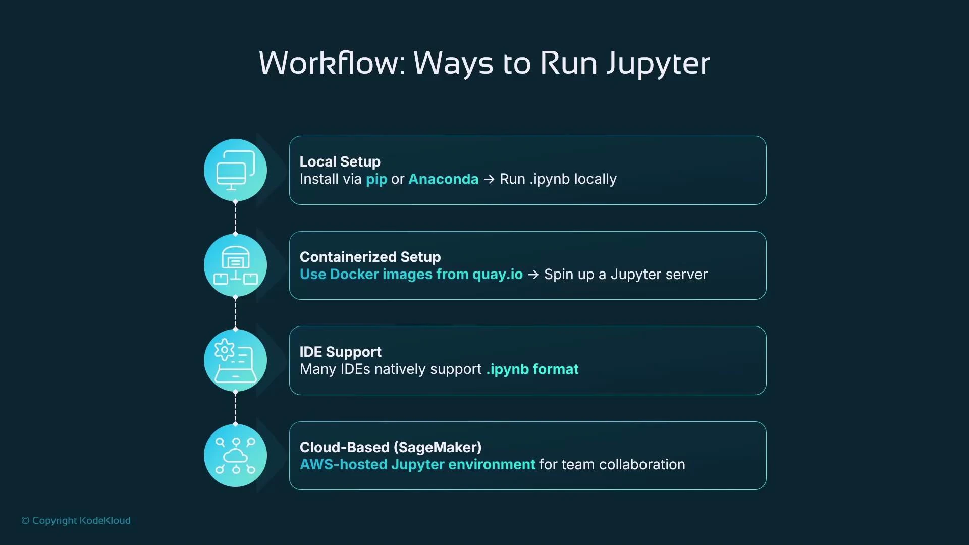
You can run Jupyter in several environments depending on your workflow, collaboration needs, and infrastructure:
| Method | When to use | Examples / Notes |
| -------------------- | ----------------------------------------------------- | ----------------------------------------------------------- |
| Local installation | Development, quick experimentation, or offline work | Install with pip or use the Anaconda distribution |
| Containerized | Isolated, reproducible environments; consistent CI/CD | Run Jupyter inside Docker images from Docker Hub or quay.io |
| Inside an IDE | Tight editor integration and local debugging | VS Code supports .ipynb files natively |
| Hosted cloud service | Scalable, managed compute and collaboration | AWS SageMaker, Google Colab, Databricks |
* Local setup
* If Python is installed, use pip:
```bash theme={null}
pip install notebook # classic Jupyter Notebook server
pip install jupyterlab # modern JupyterLab interface
```
* Or install the Anaconda distribution, which bundles Python, Jupyter, common data science libraries, and the conda package manager: [https://www.anaconda.com/products/distribution](https://www.anaconda.com/products/distribution)
* Containerized
* Use Docker or another container runtime to pull ready-made Jupyter images. Containers isolate the notebook server and dependencies from the host OS while providing the same browser-based UI.
* Inside an IDE
* Some IDEs (for example Visual Studio Code) open .ipynb files natively and provide notebook-like experiences directly inside the editor. IDE support varies; for many data-science tasks the full Jupyter UI is preferred.
* Hosted cloud service
* Managed services run Jupyter servers in the cloud and give you a remote URL to access via your browser. AWS SageMaker is a common option that integrates Jupyter/JupyterLab with AWS services and storage.
 When you run Jupyter locally or in a container, the Jupyter server exposes a web interface you open in a browser (for example [http://localhost:8888](http://localhost:8888)). With a hosted cloud service such as AWS SageMaker, your browser points to a cloud URL instead — the UI (classic Notebook or JupyterLab) looks the same but runs on managed infrastructure.
Jupyter is always accessed via a web browser. The server (local, container, or cloud) runs the code and hosts the notebook application; your browser is the client.
***
## Jupyter in AWS SageMaker
AWS SageMaker has supported hosted Jupyter environments since its initial release. Over time AWS added:
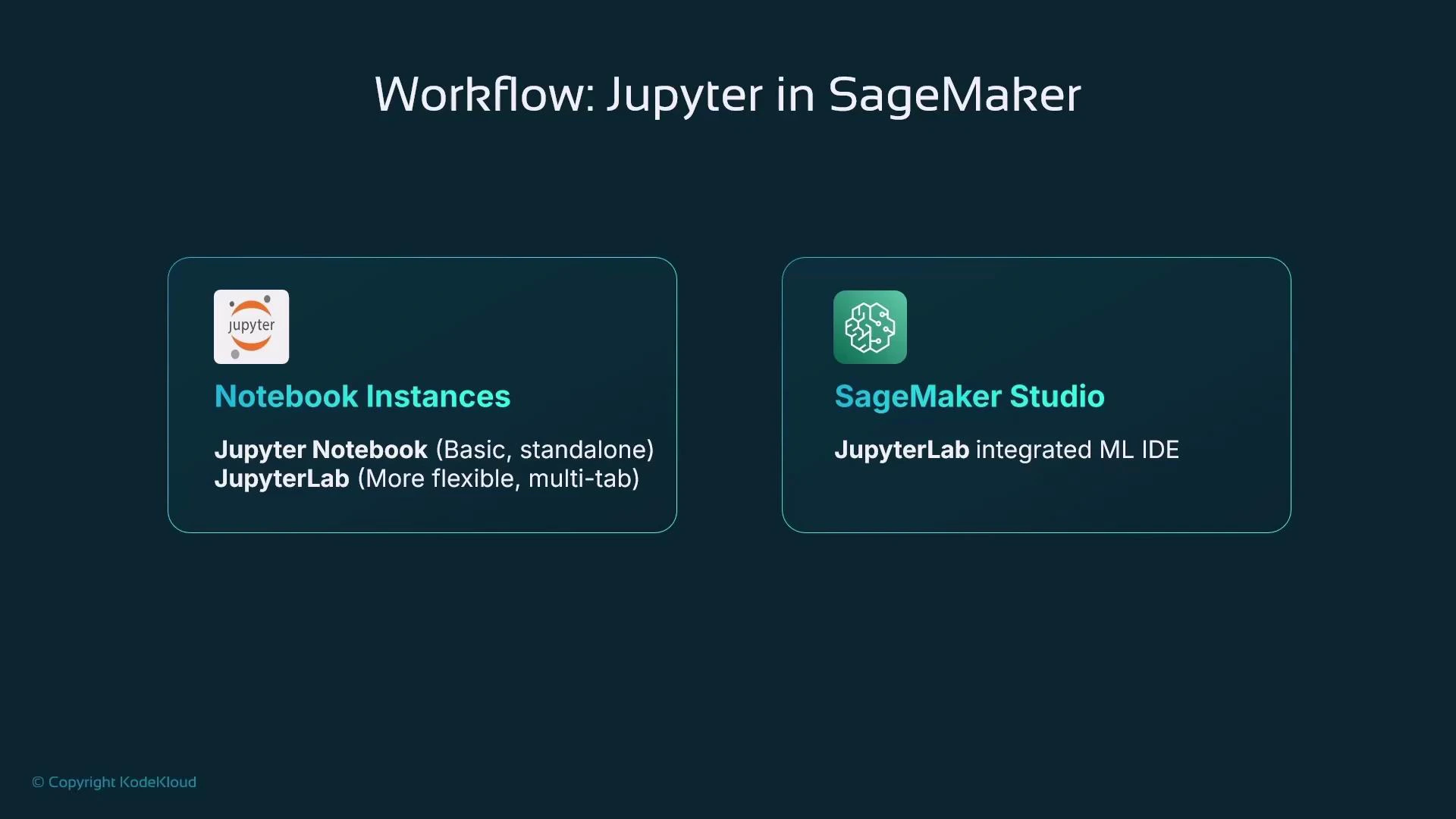
* Classic Notebook Instances — managed EC2 instances preconfigured to run a Jupyter server.
* JupyterLab support — a multi-tabbed interface with extension support.
* SageMaker Studio — a full ML-focused IDE built on JupyterLab that integrates many additional tools and workflows for data scientists and MLOps engineers.
Most new projects use SageMaker Studio because it provides a richer integrated environment beyond basic JupyterLab. SageMaker still supports legacy Notebook Instances for backward compatibility, but Studio is the recommended choice for new work.
When you run Jupyter locally or in a container, the Jupyter server exposes a web interface you open in a browser (for example [http://localhost:8888](http://localhost:8888)). With a hosted cloud service such as AWS SageMaker, your browser points to a cloud URL instead — the UI (classic Notebook or JupyterLab) looks the same but runs on managed infrastructure.
Jupyter is always accessed via a web browser. The server (local, container, or cloud) runs the code and hosts the notebook application; your browser is the client.
***
## Jupyter in AWS SageMaker
AWS SageMaker has supported hosted Jupyter environments since its initial release. Over time AWS added:
* Classic Notebook Instances — managed EC2 instances preconfigured to run a Jupyter server.
* JupyterLab support — a multi-tabbed interface with extension support.
* SageMaker Studio — a full ML-focused IDE built on JupyterLab that integrates many additional tools and workflows for data scientists and MLOps engineers.
Most new projects use SageMaker Studio because it provides a richer integrated environment beyond basic JupyterLab. SageMaker still supports legacy Notebook Instances for backward compatibility, but Studio is the recommended choice for new work.
 Notebook Instances in AWS SageMaker are supported but considered legacy. For new projects, prefer SageMaker Studio for a modern, integrated JupyterLab-based experience.
***
## Hosting resources and instance sizing
When creating a hosted Jupyter server (Notebook Instance or a Studio kernel/compute), you choose a compute profile. SageMaker uses instance families and sizes similar to EC2 naming:
| Component | Meaning |
| -------------: | ---------------------------------------------------------------------------------------- |
| Family | Workload type (M = general purpose, C = compute-optimized, P = GPU/accelerated) |
| Generation | Newer generations (e.g., M6) use more recent CPU/GPU hardware than older ones (M5, etc.) |
| Size (t-shirt) | CPU / memory / GPU capacity (large, xlarge, 2xlarge, etc.) |
Choose an instance type that matches your workloads: data preprocessing, model training, or GPU-accelerated deep learning. You can provision multiple hosted environments with different sizes for different projects.
When you run cells inside a notebook, code executes on the server. Notebook cells capture stdout and visual outputs inline and save them into the .ipynb document.
Example notebook cells:
```python theme={null}
# Example 1: Simple arithmetic in a notebook cell
a = 10
b = 5
print(a + b)
# Output:
# 15
```
```python theme={null}
# Example 2: Iterate over a list of prices and print each
prices = [50000, 60000, 65000, 44000, 127000]
for price in prices:
print(f'Current price is {price}')
# Output:
# Current price is 50000
# Current price is 60000
# Current price is 65000
# Current price is 44000
# Current price is 127000
```
***
## Visualizations and documentation
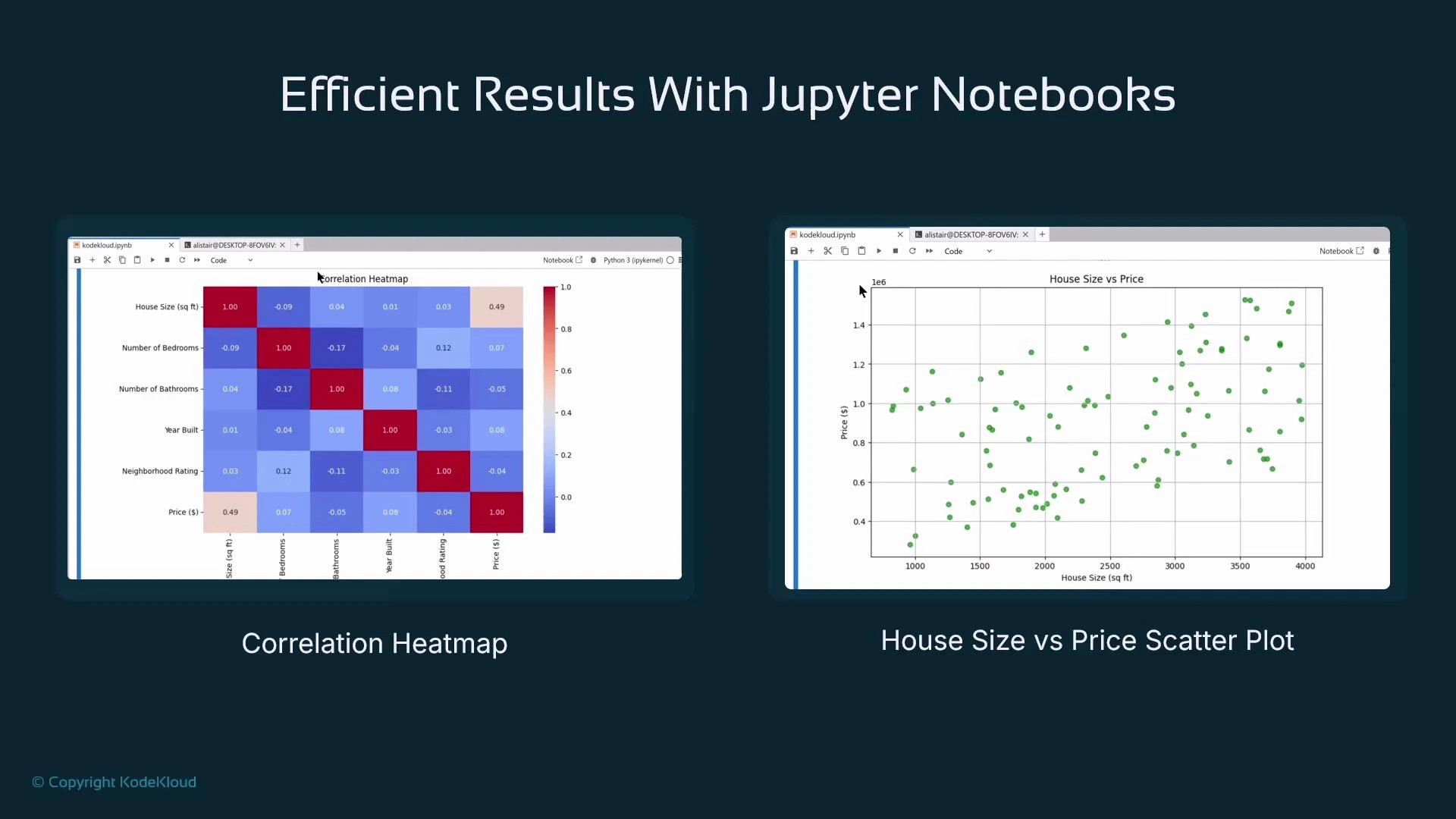
A major strength of Jupyter is inline rendering of visualizations. Libraries such as Matplotlib and Seaborn render charts and plots directly into notebook output cells. These visual outputs are preserved in the .ipynb file (unless cleared), which makes notebooks ideal for combining code, visual results, and narrative in one shareable document.
Common visualization types used in data science:
| Visualization | Use case |
| --------------------------------- | ------------------------------------------------------------------------------- |
| Correlation heatmap | Understand relationships between numeric features; useful for feature selection |
| Scatter plot | Inspect relationships and outliers (e.g., house size vs. price) |
| Line charts, histograms, boxplots | Time series, distributions, and data summaries |
Notebook Instances in AWS SageMaker are supported but considered legacy. For new projects, prefer SageMaker Studio for a modern, integrated JupyterLab-based experience.
***
## Hosting resources and instance sizing
When creating a hosted Jupyter server (Notebook Instance or a Studio kernel/compute), you choose a compute profile. SageMaker uses instance families and sizes similar to EC2 naming:
| Component | Meaning |
| -------------: | ---------------------------------------------------------------------------------------- |
| Family | Workload type (M = general purpose, C = compute-optimized, P = GPU/accelerated) |
| Generation | Newer generations (e.g., M6) use more recent CPU/GPU hardware than older ones (M5, etc.) |
| Size (t-shirt) | CPU / memory / GPU capacity (large, xlarge, 2xlarge, etc.) |
Choose an instance type that matches your workloads: data preprocessing, model training, or GPU-accelerated deep learning. You can provision multiple hosted environments with different sizes for different projects.
When you run cells inside a notebook, code executes on the server. Notebook cells capture stdout and visual outputs inline and save them into the .ipynb document.
Example notebook cells:
```python theme={null}
# Example 1: Simple arithmetic in a notebook cell
a = 10
b = 5
print(a + b)
# Output:
# 15
```
```python theme={null}
# Example 2: Iterate over a list of prices and print each
prices = [50000, 60000, 65000, 44000, 127000]
for price in prices:
print(f'Current price is {price}')
# Output:
# Current price is 50000
# Current price is 60000
# Current price is 65000
# Current price is 44000
# Current price is 127000
```
***
## Visualizations and documentation
A major strength of Jupyter is inline rendering of visualizations. Libraries such as Matplotlib and Seaborn render charts and plots directly into notebook output cells. These visual outputs are preserved in the .ipynb file (unless cleared), which makes notebooks ideal for combining code, visual results, and narrative in one shareable document.
Common visualization types used in data science:
| Visualization | Use case |
| --------------------------------- | ------------------------------------------------------------------------------- |
| Correlation heatmap | Understand relationships between numeric features; useful for feature selection |
| Scatter plot | Inspect relationships and outliers (e.g., house size vs. price) |
| Line charts, histograms, boxplots | Time series, distributions, and data summaries |
 Benefits of using Jupyter for data science:
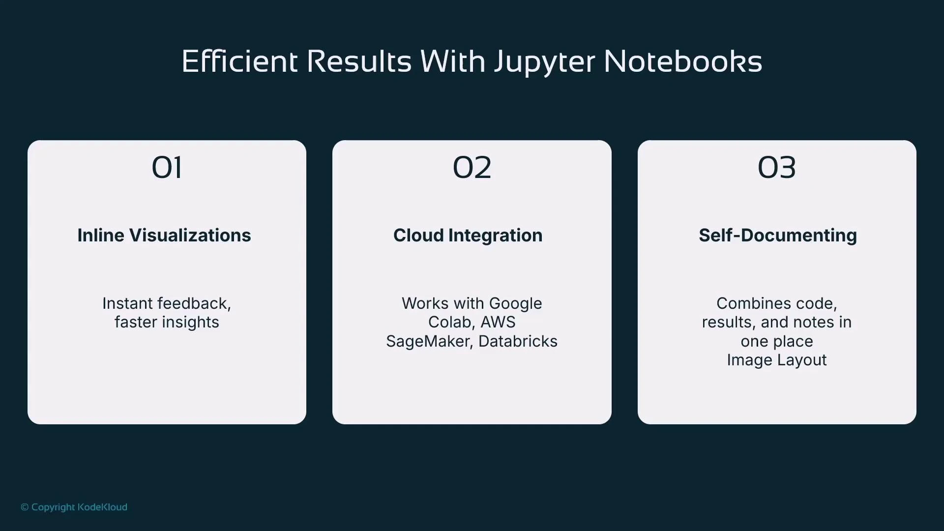
* Inline visualizations and instant feedback from code execution.
* Integration with many cloud environments (e.g., Google Colab, AWS SageMaker, Databricks).
* Self-documenting workflows: combine code cells with markdown for clear explanations, hypotheses, and reproducible steps.
Benefits of using Jupyter for data science:
* Inline visualizations and instant feedback from code execution.
* Integration with many cloud environments (e.g., Google Colab, AWS SageMaker, Databricks).
* Self-documenting workflows: combine code cells with markdown for clear explanations, hypotheses, and reproducible steps.
 Jupyter is widely used across industry (for example Airbnb, NASA, and Netflix) for exploratory analysis, model development, and collaborative data science projects.
***
## Summary
Key takeaways from this lesson:
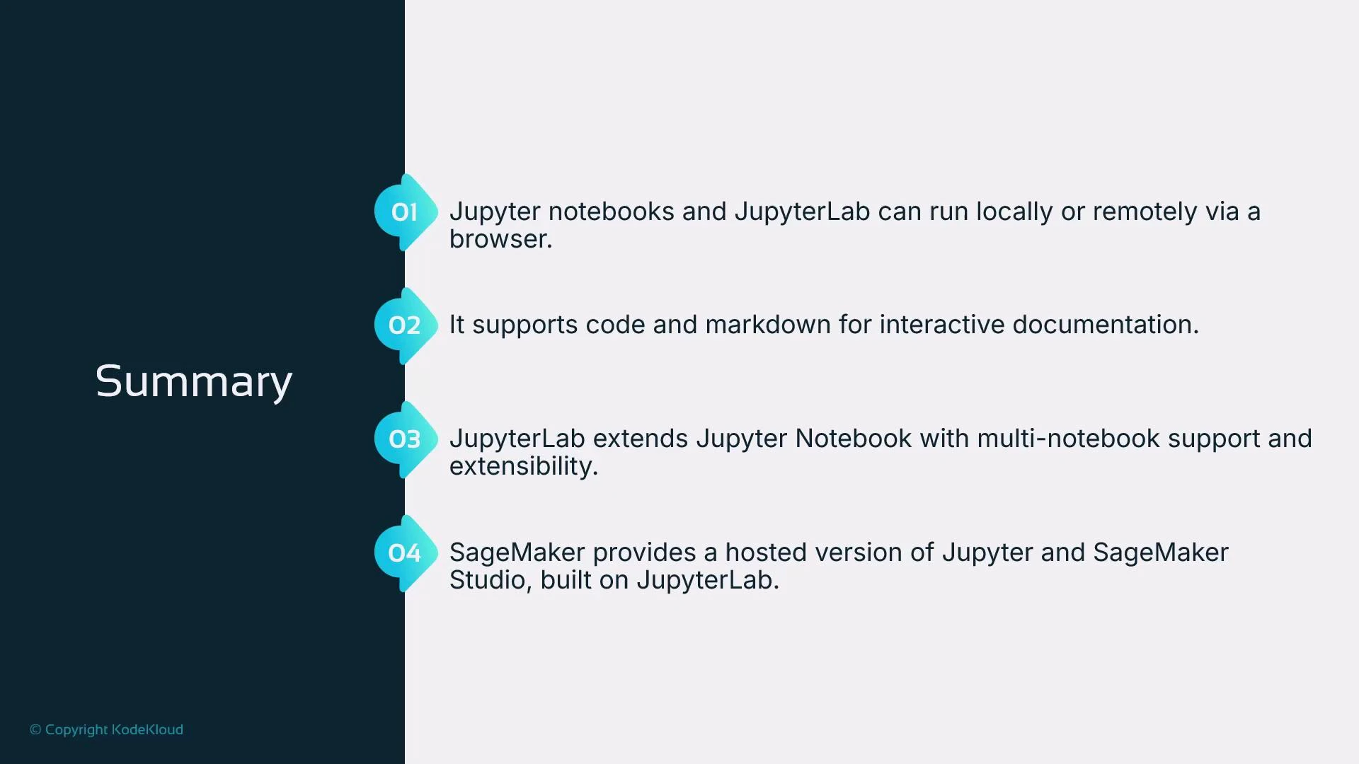
* Ways to run Jupyter: locally (pip or Anaconda), in containers, inside IDEs, or as hosted cloud services (e.g., AWS SageMaker).
* The browser is always the user interface for Jupyter; the server executes code and stores outputs.
* Notebook cells can be code or markdown; code cell stdout and visual outputs are captured inline in the .ipynb file.
* JupyterLab is a modern, tabbed interface with extension support; SageMaker Studio builds on JupyterLab to provide a full ML IDE.
* SageMaker supports legacy Notebook Instances and the newer Studio — prefer Studio for new projects.
Jupyter is widely used across industry (for example Airbnb, NASA, and Netflix) for exploratory analysis, model development, and collaborative data science projects.
***
## Summary
Key takeaways from this lesson:
* Ways to run Jupyter: locally (pip or Anaconda), in containers, inside IDEs, or as hosted cloud services (e.g., AWS SageMaker).
* The browser is always the user interface for Jupyter; the server executes code and stores outputs.
* Notebook cells can be code or markdown; code cell stdout and visual outputs are captured inline in the .ipynb file.
* JupyterLab is a modern, tabbed interface with extension support; SageMaker Studio builds on JupyterLab to provide a full ML IDE.
* SageMaker supports legacy Notebook Instances and the newer Studio — prefer Studio for new projects.
 A hands-on demo using JupyterLab in AWS SageMaker Studio will be provided later in the course.
## Links and references
* JupyterLab: [https://jupyter.org/](https://jupyter.org/)
* Anaconda distribution: [https://www.anaconda.com/products/distribution](https://www.anaconda.com/products/distribution)
* Docker: [https://www.docker.com/](https://www.docker.com/)
* AWS SageMaker overview and resources: [https://learn.kodekloud.com/user/courses/aws-sagemaker](https://learn.kodekloud.com/user/courses/aws-sagemaker)
* Matplotlib: [https://matplotlib.org/](https://matplotlib.org/)
* Seaborn: [https://seaborn.pydata.org/](https://seaborn.pydata.org/)
A hands-on demo using JupyterLab in AWS SageMaker Studio will be provided later in the course.
## Links and references
* JupyterLab: [https://jupyter.org/](https://jupyter.org/)
* Anaconda distribution: [https://www.anaconda.com/products/distribution](https://www.anaconda.com/products/distribution)
* Docker: [https://www.docker.com/](https://www.docker.com/)
* AWS SageMaker overview and resources: [https://learn.kodekloud.com/user/courses/aws-sagemaker](https://learn.kodekloud.com/user/courses/aws-sagemaker)
* Matplotlib: [https://matplotlib.org/](https://matplotlib.org/)
* Seaborn: [https://seaborn.pydata.org/](https://seaborn.pydata.org/)