Demo Setup MLflow server and run the ML Experiment

Welcome to this guide on setting up an MLflow server and running an end-to-end machine learning experiment. In this demo, we simulate health insurance claims data (with injected anomalies) and build an anomaly detection model using the Isolation Forest algorithm. Follow along to set up your MLflow server in VS Code, generate synthetic data, train a model, and log results to MLflow.

1. Setting Up MLflow

Begin by launching the MLflow UI. Open the terminal in VS Code and run:

mlflow ui

After executing the command, MLflow will start, and a pop-up notification should appear. Click on "open browser" to verify that the MLflow web UI is accessible. Once confirmed, create a new terminal in VS Code to continue with the next steps.

2. Generating Synthetic Data

If you haven't already generated the synthetic data, run the provided script. This script simulates health insurance claims, including some injected anomalies. Create a file named synthetic_health_claims.py and add the following content:

import pandas as pd
import numpy as np

# Assume 'data' and 'num_samples' are defined previously in your project
df = pd.DataFrame(data)

# Introduce some anomalies (e.g., very high claim amounts)
num_anomalies = 50
anomalies = {
    'claim_id': np.arange(num_samples + 1, num_samples + num_anomalies + 1),
    'claim_amount': np.random.randint(10000, 25000, num_anomalies),  # Much higher amounts
    'patient_age': np.random.randint(18, 90, num_anomalies),
    'provider_id': np.random.randint(1, 50, num_anomalies),
    'days_since_last_claim': np.random.randint(0, 365, num_anomalies)
}

df_anomalies = pd.DataFrame(anomalies)

# Combine normal data with anomalies
df = pd.concat([df, df_anomalies]).reset_index(drop=True)

# Shuffle the dataset
df = df.sample(frac=1).reset_index(drop=True)

# Save the data to CSV
df.to_csv('synthetic_health_claims.csv', index=False)

Run the script using the following command:

python3 synthetic_health_claims.py

Upon execution, you should see an output confirming that the synthetic data was generated and saved. The console output will also show that the MLflow UI is running, along with relevant log messages.

3. Creating and Running the ML Experiment

In this section, you'll train an ML model to perform anomaly detection using the Isolation Forest algorithm and log experiment details to the MLflow server.

Step 3.1: Model Training Script

Create a file named isolation_model.py with the following content:

import pandas as pd
from sklearn.ensemble import IsolationForest
from sklearn.model_selection import train_test_split
import mlflow
import mlflow.sklearn

# Load the synthetic data
df = pd.read_csv('synthetic_health_claims.csv')

# Set the MLflow tracking URI
mlflow.set_tracking_uri("http://127.0.0.1:5000")

# Define the features for the model. Note that 'claim_id' is not used.
features = ['claim_amount', 'num_services', 'patient_age', 'provider_id', 'days_since_last_claim']

# Split the data into training and test sets
X_train, X_test = train_test_split(df[features], test_size=0.2, random_state=42)

# Create (or set) the experiment in MLflow
mlflow.set_experiment("Health Insurance Claim Anomaly Detection")

with mlflow.start_run():
    # Train the Isolation Forest model
    model = IsolationForest(n_estimators=100, contamination=0.05, random_state=42)
    model.fit(X_train)

    # Predict anomalies on training and test sets
    y_pred_train = model.predict(X_train)
    y_pred_test = model.predict(X_test)

    # Calculate the percentage of detected anomalies
    train_anomaly_percentage = (y_pred_train == -1).mean() * 100
    test_anomaly_percentage = (y_pred_test == -1).mean() * 100

    # Log model parameters
    mlflow.log_param("n_estimators", 100)
    mlflow.log_param("contamination", 0.05)

    # Log computed metrics
    mlflow.log_metric("train_anomaly_percentage", train_anomaly_percentage)
    mlflow.log_metric("test_anomaly_percentage", test_anomaly_percentage)

    # Log the model artifact to MLflow
    mlflow.sklearn.log_model(model, "model")

    print(f"Train Anomaly Percentage: {train_anomaly_percentage:.2f}%")
    print(f"Test Anomaly Percentage: {test_anomaly_percentage:.2f}%")
    print("Model and metrics logged to MLflow.")

Run the script by executing:

python3 isolation_model.py

The terminal will display detailed output regarding the experiment, including logged parameters and metrics. A typical output snippet might look like this:

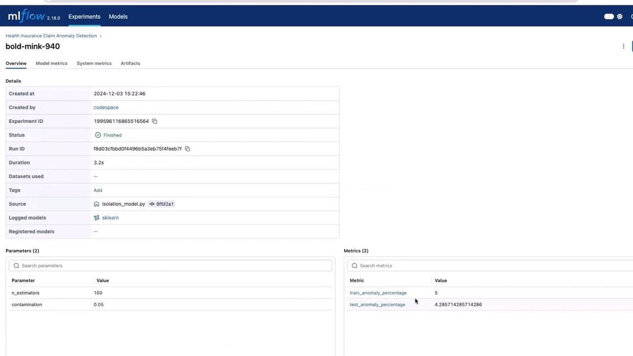
2024/12/03 11:22:46 INFO mlflow.tracking.fluent: Experiment with name 'Health Insurance Claim Anomaly Detection' does not exist. Creating a new experiment.
2024/12/03 11:22:46 WARNING mlflow.models.model: Model logged without a signature and input example. Please set `input_example` parameter when logging the model to auto infer the model signature.
Train Anomaly Percentage: 5.20%
Test Anomaly Percentage: 4.29%
Model and metrics logged to MLflow.
View run: http://127.0.0.1:5000/e/experiments/199596116865516564

4. Validating the Experiment in MLflow

Once the script finishes running, refresh your browser where the MLflow UI is open. You should now see the "Health Insurance Claim Anomaly Detection" experiment, complete with parameters, metrics, and the model artifact.

This UI confirms that your experiment has been successfully logged and is ready for further exploration or deployment.

5. Next Steps

In a production setting, your model may undergo multiple iterations and rigorous testing before deployment. For this demo, we directly use the output from this experiment. The logged model artifact, which might be stored as a pickle file or another format, can be downloaded from the MLflow UI and integrated further.

The next phase typically involves building a service around the model using frameworks like BentoML. For more detailed information on BentoML, refer to the BentoML Documentation.

Thank you for reading this guide on setting up the MLflow server and running your ML experiment. For additional resources, check out the following links:

• MLflow Documentation
• scikit-learn Documentation
• VS Code Documentation

Happy experimenting!