Demo Running and experiment and storing the result on MLflow

Hello and welcome back.

In this lesson, we demonstrate how to run an experiment locally and store its results in an MLflow service configured earlier. We'll use scikit-learn for this example and learn how to log key metrics, store models, and view experiments in the MLflow UI.

Let’s jump into our VS Code editor.

Preparing Your Environment

Before running any experiment, ensure you choose an appropriate use case and data science package. In this example, we use scikit-learn.

$ mlflow ui
[2024-11-05 18:33:22 +0000] [7842] [INFO] Starting gunicorn 23.0.0
[2024-11-05 18:33:22 +0000] [7842] [INFO] Listening at: http://127.0.0.1:5000 (7842)
[2024-11-05 18:33:22 +0000] [7842] [INFO] Using worker: sync
[2024-11-05 18:33:22 +0000] [7848] [INFO] Booting worker with pid: 7848
[2024-11-05 18:33:22 +0000] [7863] [INFO] Booting worker with pid: 7863
[2024-11-05 18:33:22 +0000] [7864] [INFO] Booting worker with pid: 7864

Creating the Experiment File

Create a new file named example_mlflow.py in your VS Code editor and paste the code below. This script sets the MLflow tracking URI, creates synthetic regression data, splits it into training and testing sets, and defines a helper function to train models, make predictions, log metrics, and store models in MLflow.

from sklearn.metrics import mean_squared_error, r2_score, mean_absolute_error, explained_variance_score
from sklearn.datasets import make_regression
from sklearn.model_selection import train_test_split
from sklearn.linear_model import LinearRegression
from sklearn.tree import DecisionTreeRegressor
from sklearn.ensemble import RandomForestRegressor
import mlflow
import mlflow.sklearn
import numpy as np

# Set the MLflow tracking URI to the remote MLflow server
mlflow.set_tracking_uri("http://localhost:5000")

# Create synthetic data for regression
X, y = make_regression(n_samples=100, n_features=4, noise=0.1, random_state=42)

# Split the data into training and testing sets
X_train, X_test, y_train, y_test = train_test_split(X, y, test_size=0.2, random_state=42)

# Set the experiment name in MLflow
mlflow.set_experiment("ML Model Experiment")

def log_model(model, model_name):
    with mlflow.start_run(run_name=model_name):
        # Train the model
        model.fit(X_train, y_train)
        # Make predictions
        y_pred = model.predict(X_test)
        
        # Compute key metrics
        mse = mean_squared_error(y_test, y_pred)
        rmse = np.sqrt(mse)
        mae = mean_absolute_error(y_test, y_pred)
        r2 = r2_score(y_test, y_pred)
        evs = explained_variance_score(y_test, y_pred)
        
        # Log metrics to MLflow
        mlflow.log_metric("mse", mse)
        mlflow.log_metric("rmse", rmse)
        mlflow.log_metric("mae", mae)
        mlflow.log_metric("r2", r2)
        mlflow.log_metric("explained_variance", evs)
        
        # Log the model itself
        mlflow.sklearn.log_model(model, model_name)
        
        print(f"{model_name} - MSE: {mse}, RMSE: {rmse}, MAE: {mae}, R2: {r2}, Explained Variance: {evs}")

# Linear Regression Model
linear_model = LinearRegression()
log_model(linear_model, "Linear Regression")

# Decision Tree Regressor Model
tree_model = DecisionTreeRegressor()
log_model(tree_model, "Decision Tree Regressor")

# Random Forest Regressor Model
forest_model = RandomForestRegressor()
log_model(forest_model, "Random Forest Regressor")

print("Experiment completed! Check the MLflow server for details.")

Installing Required Packages

Make sure you have scikit-learn installed. Open a new terminal session and run the following command:

$ pip install scikit-learn

You might see output similar to:

Requirement already satisfied: scikit-learn in /home/codespace/.local/lib/python3.12/site-packages (1.5.2)
Requirement already satisfied: numpy>=1.19.5 in /home/codespace/.local/lib/python3.12/site-packages (1.21.1)
Requirement already satisfied: scipy>=1.1.0 in /home/codespace/.local/lib/python3.12/site-packages (1.14.1)
Requirement already satisfied: joblib>=1.0.0 in /home/codespace/.local/lib/python3.12/site-packages (1.4.2)
Requirement already satisfied: threadpoolctl>=2.0.0 in /home/codespace/.local/lib/python3.12/site-packages (3.5.0)
[notice] A new release of pip is available: 24.2 → 24.3.1
[notice] To update, run: python3 -m pip install --upgrade pip

Once installed, run the example file with:

$ python3 example_mlflow.py

Remember: Your MLflow UI must be running (in a separate terminal) so that the experiment data logs correctly.

Analyzing Experiment Results in MLflow

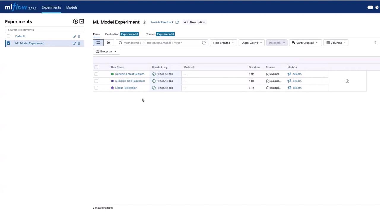
After the execution, open the MLflow UI and navigate to the experiments section to find a new experiment titled "ML Model Experiment". Here, you will see three runs corresponding to the following models:

• Linear Regression
• Decision Tree Regressor
• Random Forest Regressor

By selecting this experiment, you can view details such as run duration and input data. Use the evaluation section and select all the model runs, then click "Compare" to analyze key metrics side by side.

This comparison view provides valuable insights into the performance metrics of each model.

Another useful visualization is the contour plot, which helps compare metrics like explained variance, mean absolute error (MAE), and mean squared error (MSE) across runs.

This interface is invaluable for data science experiments, as it simplifies the process of selecting the best model based on performance metrics.

Next Steps

That concludes this lesson. In our next article, we will discuss how to store the model file in the model registry.

Thank you, and see you in the next lesson!