> ## Documentation Index
> Fetch the complete documentation index at: https://notes.kodekloud.com/llms.txt
> Use this file to discover all available pages before exploring further.
# Aggregation and Histogram
> Explains metric aggregation and histograms for summarizing telemetry, bucket types, and using percentiles to analyze distributions and detect latency outliers.
In this lesson we cover aggregation: the process of transforming raw metric samples into summarized statistics. Aggregation reduces high-volume telemetry into compact, queryable summaries that answer higher-level operational questions about your system.
 ## What is aggregation?
Aggregation takes individual measurements (for example, request latencies or current memory usage) and produces a summary such as a sum, a last-seen value, or a distribution. The aggregation type you choose determines what questions you can answer later from the stored metrics.
### Common aggregation types
| Aggregation type | Description | Typical use case |
| ---------------- | -----------------------------------------------------------: | ------------------------------------------- |
| Sum | Totals values over time to produce a cumulative measure. | `total_requests` or throughput counters. |
| Gauge | Reports the latest observed value at scrape/collection time. | Current temperature, in-progress requests. |
| Histogram | Captures the distribution of values across buckets (ranges). | Response time distributions, payload sizes. |
## What is aggregation?
Aggregation takes individual measurements (for example, request latencies or current memory usage) and produces a summary such as a sum, a last-seen value, or a distribution. The aggregation type you choose determines what questions you can answer later from the stored metrics.
### Common aggregation types
| Aggregation type | Description | Typical use case |
| ---------------- | -----------------------------------------------------------: | ------------------------------------------- |
| Sum | Totals values over time to produce a cumulative measure. | `total_requests` or throughput counters. |
| Gauge | Reports the latest observed value at scrape/collection time. | Current temperature, in-progress requests. |
| Histogram | Captures the distribution of values across buckets (ranges). | Response time distributions, payload sizes. |
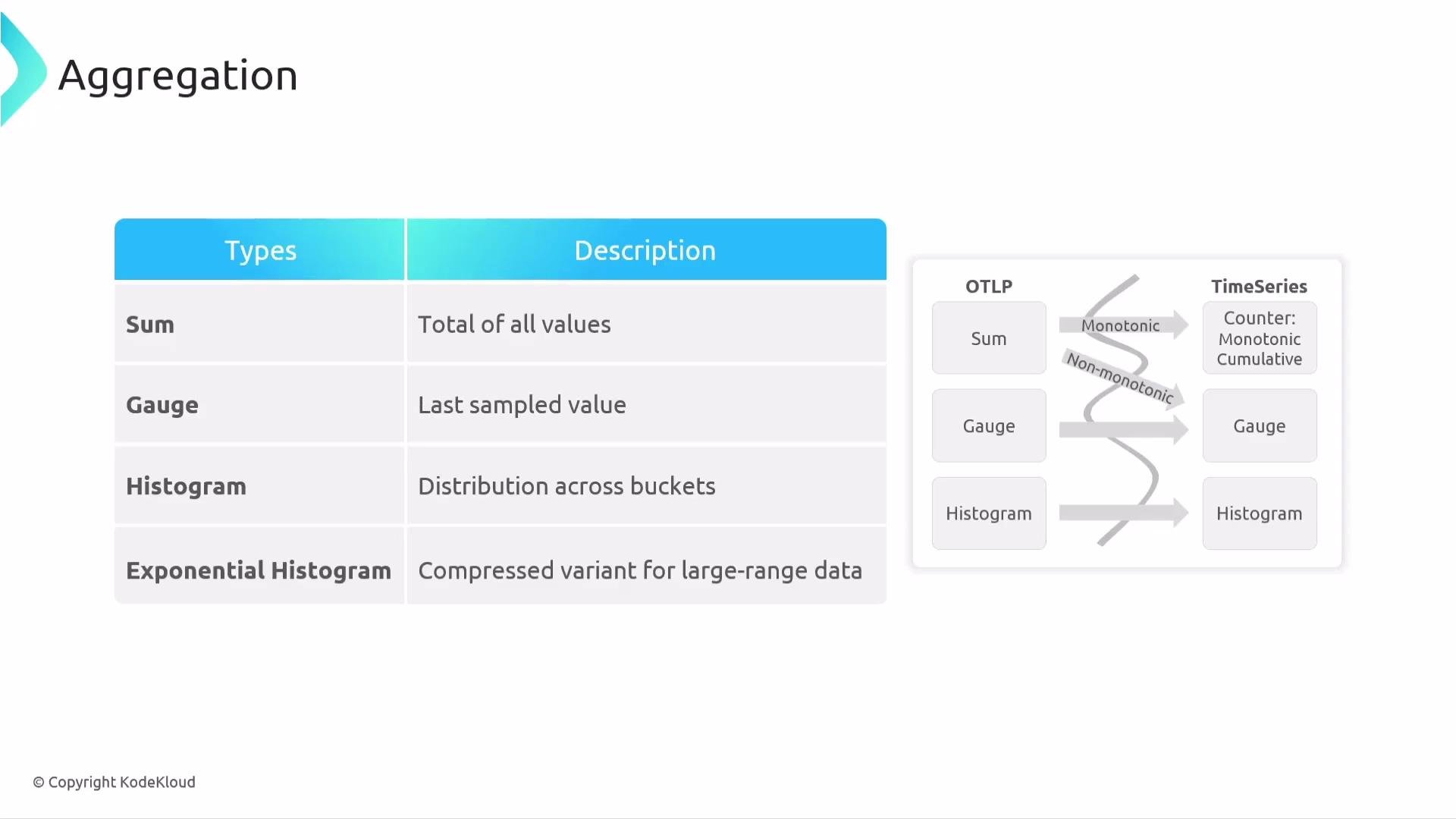 The image above also illustrates how OTLP metric types map to backend time series. Consistent mapping ensures aggregated metrics are interpreted correctly across collectors and storage backends.
## Why use histograms?
Histograms capture a distribution instead of a single scalar. This is crucial when averages hide important behavior (for example, latency spikes). Histograms let you:
* See the shape of latency or size distributions.
* Compute percentiles (P50, P95, P99) to characterize tail behavior.
* Detect and debug outliers and performance anomalies.
Exponential histograms are a compact representation that scales well for datasets with wide dynamic ranges, providing space-efficient aggregation while preserving percentile estimates.
## Example: histogram for HTTP request durations
Consider a histogram metric that tracks server request durations:
* Metric name: `http.server.duration`
* Unit: milliseconds
* Instrument type: histogram
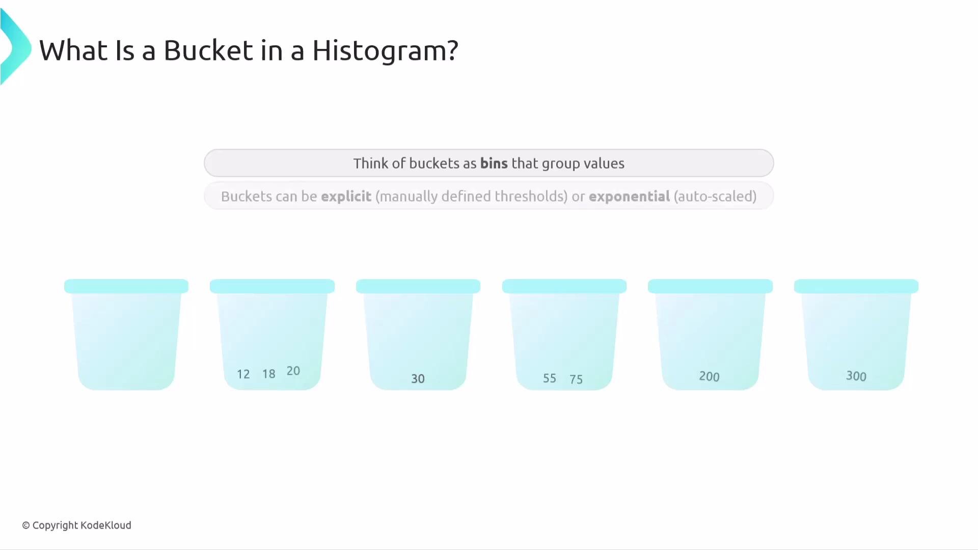
* Observed values: 12 ms, 18 ms, 20 ms, 30 ms, 75 ms, 200 ms, 300 ms
The image above also illustrates how OTLP metric types map to backend time series. Consistent mapping ensures aggregated metrics are interpreted correctly across collectors and storage backends.
## Why use histograms?
Histograms capture a distribution instead of a single scalar. This is crucial when averages hide important behavior (for example, latency spikes). Histograms let you:
* See the shape of latency or size distributions.
* Compute percentiles (P50, P95, P99) to characterize tail behavior.
* Detect and debug outliers and performance anomalies.
Exponential histograms are a compact representation that scales well for datasets with wide dynamic ranges, providing space-efficient aggregation while preserving percentile estimates.
## Example: histogram for HTTP request durations
Consider a histogram metric that tracks server request durations:
* Metric name: `http.server.duration`
* Unit: milliseconds
* Instrument type: histogram
* Observed values: 12 ms, 18 ms, 20 ms, 30 ms, 75 ms, 200 ms, 300 ms
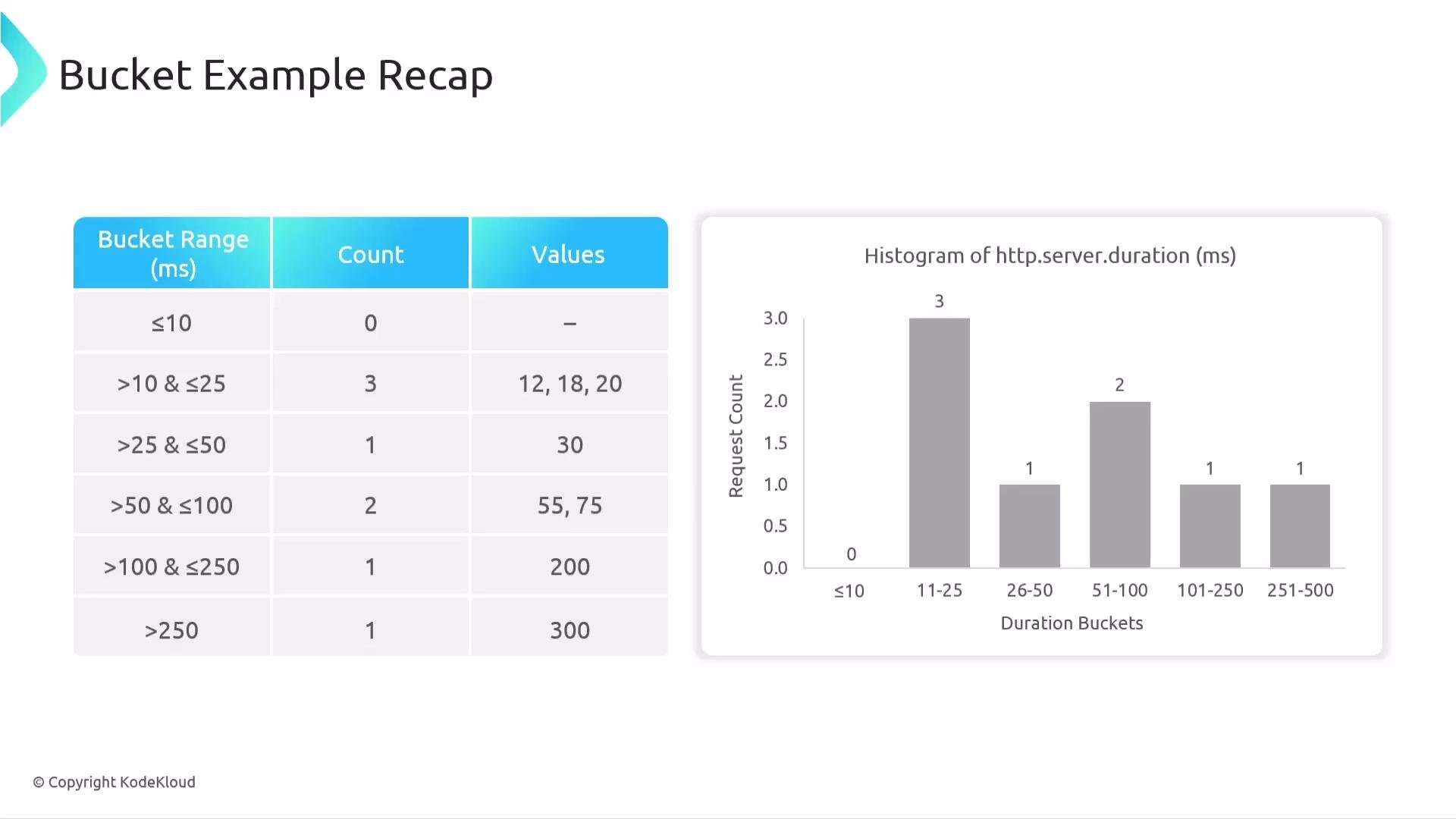
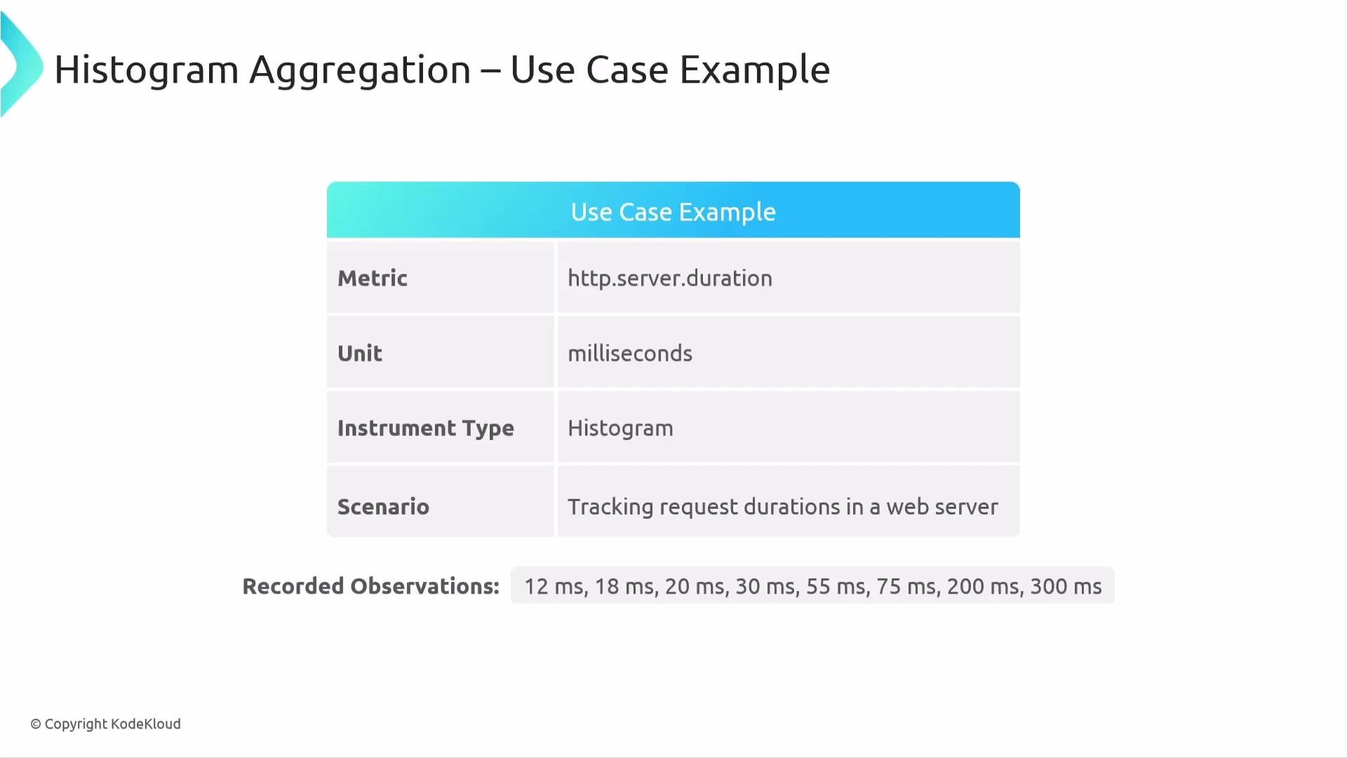 Rather than a single average, the histogram places these values into buckets (ranges) and counts how many observations fall into each one. A bucket is a contiguous range of values; the histogram records the count per bucket plus overall metadata that enables percentile estimation.
 Buckets (bins) can be configured in two common ways:
* Explicit buckets: you define threshold boundaries manually (e.g., 0–10 ms, 10–50 ms, 50–100 ms, …).
* Exponential buckets: boundaries grow exponentially and adapt better to wide-ranging values.
Buckets (bins) can be configured in two common ways:
* Explicit buckets: you define threshold boundaries manually (e.g., 0–10 ms, 10–50 ms, 50–100 ms, …).
* Exponential buckets: boundaries grow exponentially and adapt better to wide-ranging values.
 When you count recorded values into buckets, you can visualize the distribution as a bar chart and compute percentiles. For the example above, bucket counts produce a column chart that highlights that most requests are under 50 ms, a smaller group near 100 ms, and a few outliers at 300 ms.
 ### Percentiles from histograms
Percentiles summarize the distribution:
* P50 (median) — half the requests are at or below this value. In the example above: `P50 ≈ 30 ms`.
* P90 — 90% of requests are at or below this value; useful to measure typical tail latency.
* P95 and P99 — isolate heavier tails and outliers to guide performance tuning and alerting.
Use percentiles to set meaningful SLOs and to prioritize optimization efforts where tail latencies hurt user experience.
## Quick reference & resources
* OpenTelemetry Metrics overview: [https://opentelemetry.io/docs/messaging/metrics/](https://opentelemetry.io/docs/messaging/metrics/)
* Histogram guidance and best practices: check your backend docs for supported histogram types (`explicit` vs `exponential`) and percentile computation guarantees.
Histograms are essential when distribution matters. Percentiles and distribution summaries derived from histograms reveal performance characteristics that averages alone can hide.
### Percentiles from histograms
Percentiles summarize the distribution:
* P50 (median) — half the requests are at or below this value. In the example above: `P50 ≈ 30 ms`.
* P90 — 90% of requests are at or below this value; useful to measure typical tail latency.
* P95 and P99 — isolate heavier tails and outliers to guide performance tuning and alerting.
Use percentiles to set meaningful SLOs and to prioritize optimization efforts where tail latencies hurt user experience.
## Quick reference & resources
* OpenTelemetry Metrics overview: [https://opentelemetry.io/docs/messaging/metrics/](https://opentelemetry.io/docs/messaging/metrics/)
* Histogram guidance and best practices: check your backend docs for supported histogram types (`explicit` vs `exponential`) and percentile computation guarantees.
Histograms are essential when distribution matters. Percentiles and distribution summaries derived from histograms reveal performance characteristics that averages alone can hide.