> ## Documentation Index
> Fetch the complete documentation index at: https://notes.kodekloud.com/llms.txt
> Use this file to discover all available pages before exploring further.
# HistogramSummary
> Explains Prometheus histograms and summaries, meaning of _count/_sum/_bucket, PromQL queries, estimating quantiles with histogram_quantile, SLO checks, and bucket design tradeoffs
In this lesson we cover how to work with Prometheus histogram metrics in PromQL: what each submetric represents, common queries (rates, averages, percentages), how to estimate quantiles and check SLOs, and trade-offs when designing buckets versus using summaries.
A Prometheus histogram (for example, `request_latency_seconds`) exposes three kinds of time series:
| Submetric | Meaning | Example |
| --------- | --------------------------------------------------------------------- | ---------------------------------------------------------------- |
| `_count` | Total number of observations (a counter) | `request_latency_seconds_count{path="/articles"} 100` |
| `_sum` | Sum of all observed values (useful for computing averages) | `request_latency_seconds_sum{path="/articles"} 5.034496069` |
| `_bucket` | Cumulative counts per bucket boundary labeled by `le` (less-or-equal) | `request_latency_seconds_bucket{le="0.05", path="/articles"} 50` |
Here is a representative set of timeseries for a histogram:
```text theme={null}
request_latency_seconds_bucket{le="+Inf", path="/articles"} 100
request_latency_seconds_bucket{le="0.01", path="/articles"} 5
request_latency_seconds_bucket{le="0.02", path="/articles"} 17
request_latency_seconds_bucket{le="0.03", path="/articles"} 30
request_latency_seconds_bucket{le="0.04", path="/articles"} 44
request_latency_seconds_bucket{le="0.05", path="/articles"} 50
request_latency_seconds_bucket{le="0.06", path="/articles"} 64
request_latency_seconds_bucket{le="0.07", path="/articles"} 72
request_latency_seconds_bucket{le="0.08", path="/articles"} 79
request_latency_seconds_bucket{le="0.09", path="/articles"} 86
request_latency_seconds_bucket{le="0.1", path="/articles"} 100
request_latency_seconds_count{path="/articles"} 100
request_latency_seconds_sum{path="/articles"} 5.034496069
```
* `_count` (here `100`) is the total number of requests.
* `_sum` is the sum of observed latencies (seconds).
* Each `request_latency_seconds_bucket{le="X"}` is the cumulative count of observations with value ≤ X. For example `le="0.05" = 50` means 50 requests observed latency ≤ 0.05s.
Note that bucket counts are cumulative: the value at a larger `le` includes the counts of all smaller `le` buckets plus any observations between them. The `le="+Inf"` bucket should equal the `_count` series — if it does not, it usually indicates incorrect instrumentation or a bug.
Buckets are cumulative — when interpreting buckets, subtract the previous bucket if you need the number of observations that fall strictly between two boundaries.
## Common queries
Use `rate()` or `increase()` on histogram submetrics (they are counters) depending on whether you want a rate or a total increase over a range.
* Instantaneous per-second request rate (1m window):
```promql theme={null}
rate(request_latency_seconds_count[1m])
```
* Per-bucket rates (graphing bucket series over time):
```promql theme={null}
rate(request_latency_seconds_bucket[5m])
```
* Average request latency (over last 5m):
```promql theme={null}
rate(request_latency_seconds_sum[5m]) / rate(request_latency_seconds_count[5m])
```
* Fraction of requests ≤ a specific bucket (`le="0.06"`), using vector matching to ignore the `le` label on the right-hand side:
```promql theme={null}
rate(request_latency_seconds_bucket{path="/articles", le="0.06"}[5m])
/ ignoring(le) rate(request_latency_seconds_count{path="/articles"}[5m])
```
* Number of observations between two bucket boundaries (5m window):
```promql theme={null}
increase(request_latency_seconds_bucket{le="0.05", path="/articles"}[5m])
- increase(request_latency_seconds_bucket{le="0.02", path="/articles"}[5m])
```
 ## Quantiles from histograms
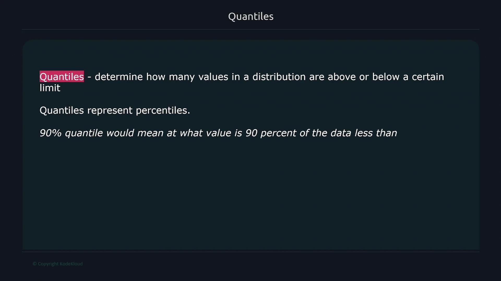
Prometheus provides `histogram_quantile()` to estimate quantiles from histogram buckets. The function takes a quantile (0..1) and a bucket series:
```promql theme={null}
histogram_quantile(0.75, request_latency_seconds_bucket)
```
When aggregating across multiple instances, aggregate bucket counters by `le` first (so the quantile function sees a complete set of bucket boundaries), for example:
```promql theme={null}
histogram_quantile(
0.95,
sum(rate(request_latency_seconds_bucket[5m])) by (le)
)
```
Example output (illustrative):
```text theme={null}
{instance="192.168.1.66:8000", job="api", method="GET", path="/articles"} 0.076
```
This indicates that \~75% of requests had latency ≤ 0.076s (estimated).
## Quantiles from histograms
Prometheus provides `histogram_quantile()` to estimate quantiles from histogram buckets. The function takes a quantile (0..1) and a bucket series:
```promql theme={null}
histogram_quantile(0.75, request_latency_seconds_bucket)
```
When aggregating across multiple instances, aggregate bucket counters by `le` first (so the quantile function sees a complete set of bucket boundaries), for example:
```promql theme={null}
histogram_quantile(
0.95,
sum(rate(request_latency_seconds_bucket[5m])) by (le)
)
```
Example output (illustrative):
```text theme={null}
{instance="192.168.1.66:8000", job="api", method="GET", path="/articles"} 0.076
```
This indicates that \~75% of requests had latency ≤ 0.076s (estimated).
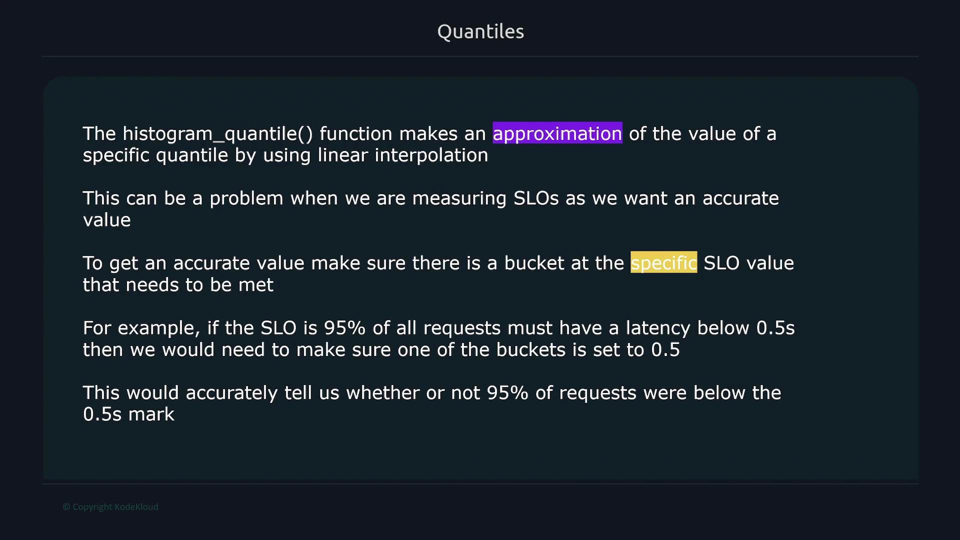 Important: `histogram_quantile()` uses linear interpolation between bucket boundaries — it produces an estimate, not an exact value. For SLO checks, ensure buckets are placed so interpolation around the SLO threshold is meaningful.
For example, if your SLO requires 95% of requests ≤ 0.5s, include a bucket at `le="0.5"` and compute:
```promql theme={null}
histogram_quantile(0.95, request_latency_seconds_bucket)
```
If the result is greater than `0.5` the SLO is missed. Keep in mind the reported quantile may be substantially influenced by bucket spacing around the threshold.
Important: `histogram_quantile()` uses linear interpolation between bucket boundaries — it produces an estimate, not an exact value. For SLO checks, ensure buckets are placed so interpolation around the SLO threshold is meaningful.
For example, if your SLO requires 95% of requests ≤ 0.5s, include a bucket at `le="0.5"` and compute:
```promql theme={null}
histogram_quantile(0.95, request_latency_seconds_bucket)
```
If the result is greater than `0.5` the SLO is missed. Keep in mind the reported quantile may be substantially influenced by bucket spacing around the threshold.
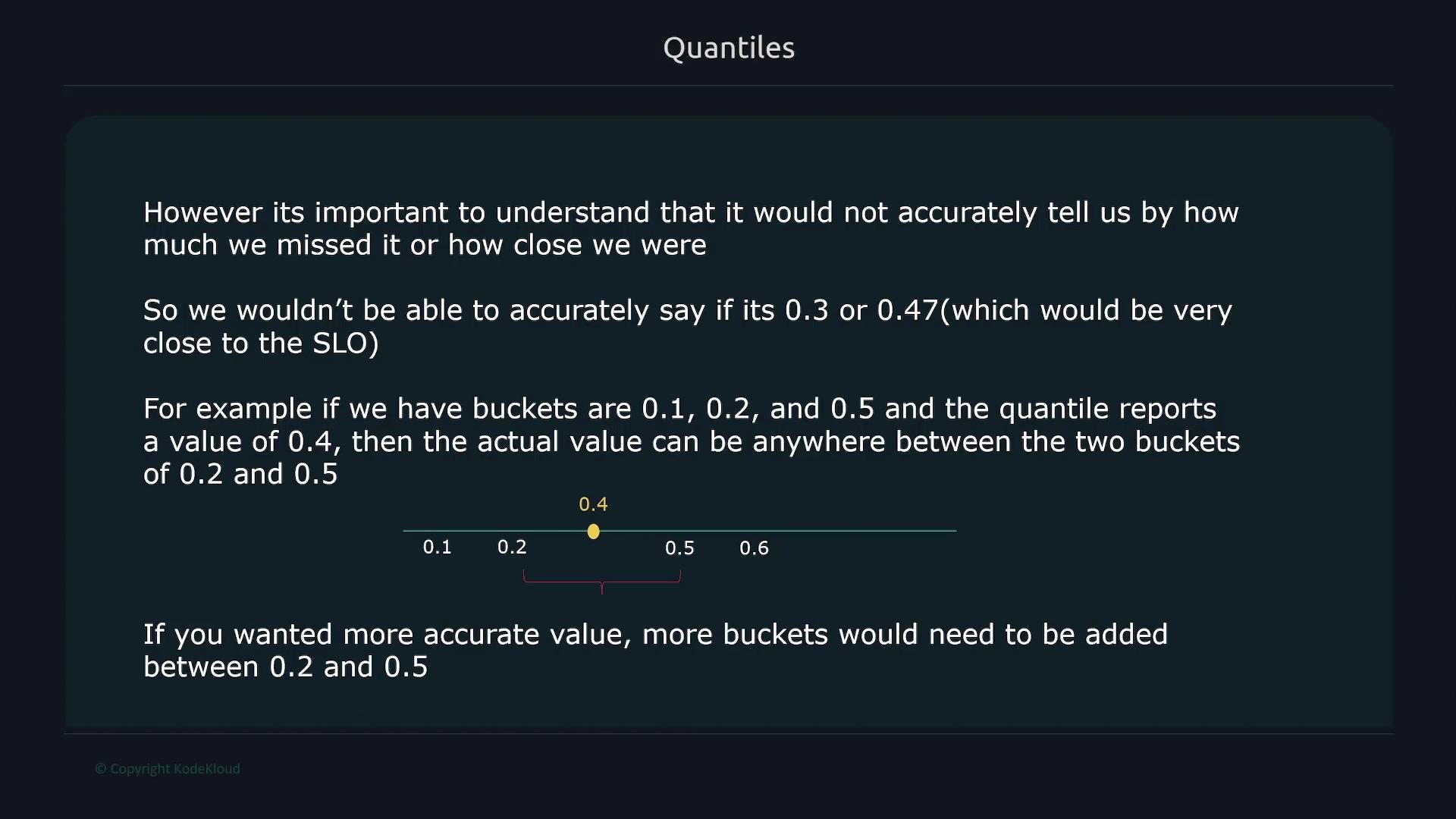 Adding more buckets improves interpolation accuracy where you need precision, but each bucket increases cardinality and Prometheus resource usage (memory, disk, and ingest cost). Choose bucket boundaries sparingly and focused around thresholds important for SLOs.
 ## Concrete histogram example
Corrected example for a `/cars` path (label order shown as `method="GET"`, `path="/cars"`):
```text theme={null}
request_latency_seconds_bucket{instance="192.168.1.168:8000", job="api", le="0.01", method="GET", path="/cars"} 2
request_latency_seconds_bucket{instance="192.168.1.168:8000", job="api", le="0.02", method="GET", path="/cars"} 3
request_latency_seconds_bucket{instance="192.168.1.168:8000", job="api", le="0.05", method="GET", path="/cars"} 5
request_latency_seconds_bucket{instance="192.168.1.168:8000", job="api", le="0.1", method="GET", path="/cars"} 6
request_latency_seconds_bucket{instance="192.168.1.168:8000", job="api", le="0.2", method="GET", path="/cars"} 10
request_latency_seconds_bucket{instance="192.168.1.168:8000", job="api", le="0.5", method="GET", path="/cars"} 14
request_latency_seconds_bucket{instance="192.168.1.168:8000", job="api", le="1", method="GET", path="/cars"} 15
request_latency_seconds_bucket{instance="192.168.1.168:8000", job="api", le="2", method="GET", path="/cars"} 18
request_latency_seconds_bucket{instance="192.168.1.168:8000", job="api", le="5", method="GET", path="/cars"} 31
request_latency_seconds_bucket{instance="192.168.1.168:8000", job="api", le="10", method="GET", path="/cars"} 57
request_latency_seconds_bucket{instance="192.168.1.168:8000", job="api", le="20", method="GET", path="/cars"} 89
request_latency_seconds_bucket{instance="192.168.1.168:8000", job="api", le="50", method="GET", path="/cars"} 99
request_latency_seconds_bucket{instance="192.168.1.168:8000", job="api", le="+Inf", method="GET", path="/cars"} 100
request_latency_seconds_count{instance="192.168.1.168:8000", job="api", method="GET", path="/cars"} 100
request_latency_seconds_sum{instance="192.168.1.168:8000", job="api", method="GET", path="/cars"} 50.0
```
* `le="0.02" = 3` → 3 requests ≤ 0.02s.
* `le="0.05" = 5` → 5 requests ≤ 0.05s (includes those ≤ 0.02s).
Compute the 95th percentile from these buckets:
```promql theme={null}
histogram_quantile(0.95, request_latency_seconds_bucket{path="/cars"})
```
Example result (illustrative):
```text theme={null}
0.96
```
This estimate implies 95% of requests had latency ≤ 0.96s given the bucket placement and interpolation.
## Summaries vs Histograms
A Prometheus summary (client-side summary) exposes quantiles directly rather than buckets. A summary typically provides:
* `request_latency_seconds{quantile="0.01"} 0.004`
* `request_latency_seconds{quantile="0.5"} 0.0296`
* `request_latency_seconds{quantile="0.95"} 0.06`
* `request_latency_seconds_count` — total samples
* `request_latency_seconds_sum` — sum of observed values
Example:
```text theme={null}
request_latency_seconds{path="/articles", quantile="0.01"} 0.004
request_latency_seconds{path="/articles", quantile="0.1"} 0.0114
request_latency_seconds{path="/articles", quantile="0.5"} 0.0296
request_latency_seconds{path="/articles", quantile="0.9"} 0.05325
request_latency_seconds{path="/articles", quantile="0.95"} 0.06
request_latency_seconds_count{path="/articles"} 100
request_latency_seconds_sum{path="/articles"} 3.144
```
Summaries return client-computed quantiles (no server interpolation), but you must decide which quantiles to record at instrumentation time and aggregation across instances is limited.
## Concrete histogram example
Corrected example for a `/cars` path (label order shown as `method="GET"`, `path="/cars"`):
```text theme={null}
request_latency_seconds_bucket{instance="192.168.1.168:8000", job="api", le="0.01", method="GET", path="/cars"} 2
request_latency_seconds_bucket{instance="192.168.1.168:8000", job="api", le="0.02", method="GET", path="/cars"} 3
request_latency_seconds_bucket{instance="192.168.1.168:8000", job="api", le="0.05", method="GET", path="/cars"} 5
request_latency_seconds_bucket{instance="192.168.1.168:8000", job="api", le="0.1", method="GET", path="/cars"} 6
request_latency_seconds_bucket{instance="192.168.1.168:8000", job="api", le="0.2", method="GET", path="/cars"} 10
request_latency_seconds_bucket{instance="192.168.1.168:8000", job="api", le="0.5", method="GET", path="/cars"} 14
request_latency_seconds_bucket{instance="192.168.1.168:8000", job="api", le="1", method="GET", path="/cars"} 15
request_latency_seconds_bucket{instance="192.168.1.168:8000", job="api", le="2", method="GET", path="/cars"} 18
request_latency_seconds_bucket{instance="192.168.1.168:8000", job="api", le="5", method="GET", path="/cars"} 31
request_latency_seconds_bucket{instance="192.168.1.168:8000", job="api", le="10", method="GET", path="/cars"} 57
request_latency_seconds_bucket{instance="192.168.1.168:8000", job="api", le="20", method="GET", path="/cars"} 89
request_latency_seconds_bucket{instance="192.168.1.168:8000", job="api", le="50", method="GET", path="/cars"} 99
request_latency_seconds_bucket{instance="192.168.1.168:8000", job="api", le="+Inf", method="GET", path="/cars"} 100
request_latency_seconds_count{instance="192.168.1.168:8000", job="api", method="GET", path="/cars"} 100
request_latency_seconds_sum{instance="192.168.1.168:8000", job="api", method="GET", path="/cars"} 50.0
```
* `le="0.02" = 3` → 3 requests ≤ 0.02s.
* `le="0.05" = 5` → 5 requests ≤ 0.05s (includes those ≤ 0.02s).
Compute the 95th percentile from these buckets:
```promql theme={null}
histogram_quantile(0.95, request_latency_seconds_bucket{path="/cars"})
```
Example result (illustrative):
```text theme={null}
0.96
```
This estimate implies 95% of requests had latency ≤ 0.96s given the bucket placement and interpolation.
## Summaries vs Histograms
A Prometheus summary (client-side summary) exposes quantiles directly rather than buckets. A summary typically provides:
* `request_latency_seconds{quantile="0.01"} 0.004`
* `request_latency_seconds{quantile="0.5"} 0.0296`
* `request_latency_seconds{quantile="0.95"} 0.06`
* `request_latency_seconds_count` — total samples
* `request_latency_seconds_sum` — sum of observed values
Example:
```text theme={null}
request_latency_seconds{path="/articles", quantile="0.01"} 0.004
request_latency_seconds{path="/articles", quantile="0.1"} 0.0114
request_latency_seconds{path="/articles", quantile="0.5"} 0.0296
request_latency_seconds{path="/articles", quantile="0.9"} 0.05325
request_latency_seconds{path="/articles", quantile="0.95"} 0.06
request_latency_seconds_count{path="/articles"} 100
request_latency_seconds_sum{path="/articles"} 3.144
```
Summaries return client-computed quantiles (no server interpolation), but you must decide which quantiles to record at instrumentation time and aggregation across instances is limited.
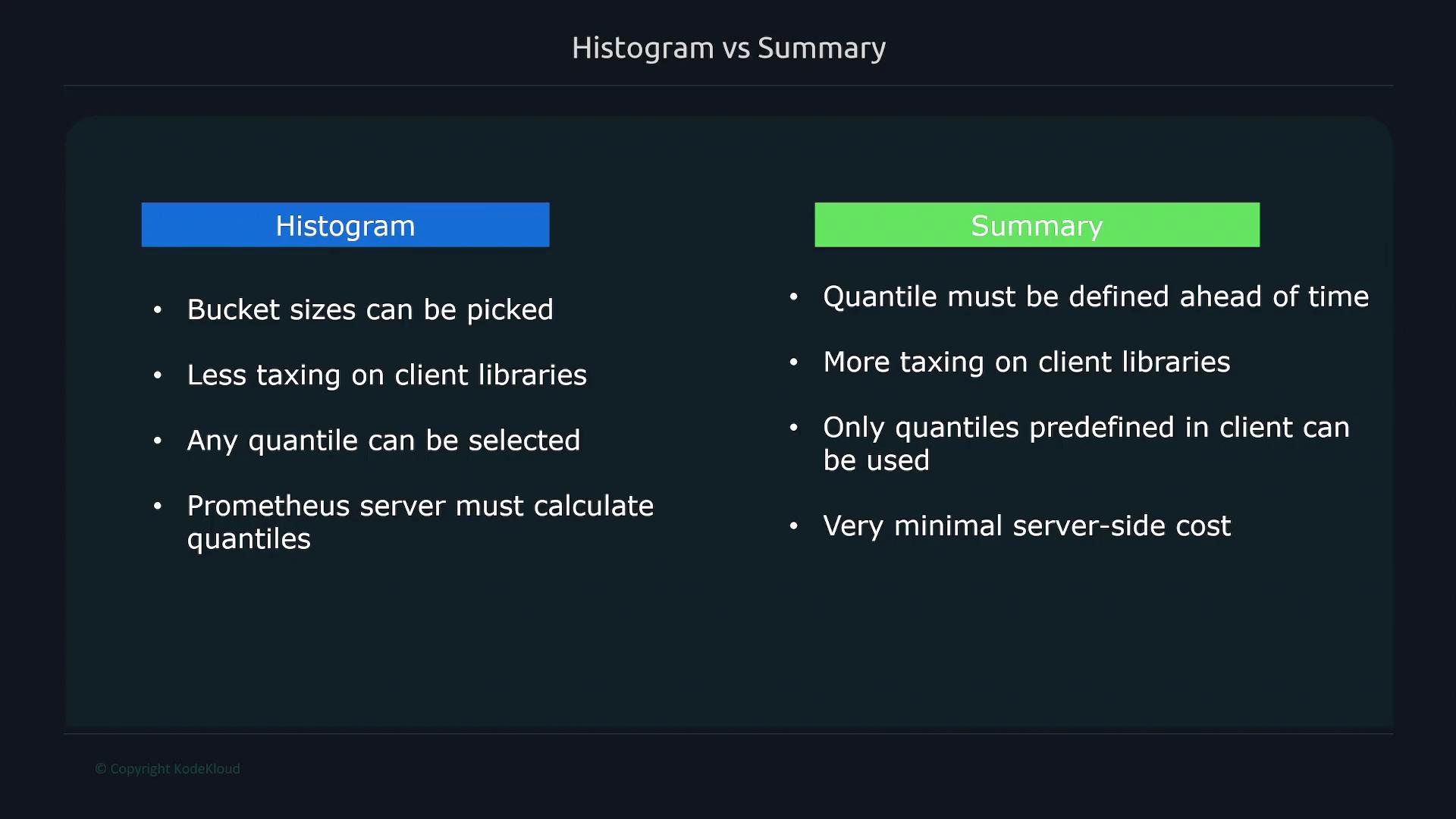 ## Design trade-offs
| Aspect | Histograms | Summaries |
| ---------------------------- | ----------------------------------------------------------------------------------: | -------------------------------------------------------------------------------- |
| Quantiles | Server-side approximate via `histogram_quantile()` (any quantile) | Client-side precomputed quantiles (exact-ish for algorithm) |
| Bucket/quantile selection | Buckets chosen at instrumentation; can compute any quantile server-side | Must choose quantiles at instrumentation time |
| Aggregation across instances | Easy—aggregate buckets by `le` then compute quantile | Harder—client quantiles don't combine well across instances |
| Cardinality & resource cost | High if many buckets (memory & disk) | Lower on server, more client CPU/memory |
| Use case | Best when you need flexible, aggregated quantiles and can afford bucket cardinality | Best when you know the exact quantiles needed and prefer client-side computation |
Keep these trade-offs in mind when designing metrics and SLO checks.
If your SLO depends on a specific latency threshold, add a bucket exactly at that threshold (or have buckets tightly spaced around it). Otherwise `histogram_quantile()` can only estimate and might hide how close you are to the SLO boundary.
## References and further reading
* [Prometheus: Histogram and Summary](https://prometheus.io/docs/practices/histograms/)
* [PromQL: histogram\_quantile() documentation](https://prometheus.io/docs/prometheus/latest/querying/functions/#histogram_quantile)
Keep bucket cardinality focused on the thresholds and percentiles that matter for your SLOs to balance accuracy and resource usage.
## Design trade-offs
| Aspect | Histograms | Summaries |
| ---------------------------- | ----------------------------------------------------------------------------------: | -------------------------------------------------------------------------------- |
| Quantiles | Server-side approximate via `histogram_quantile()` (any quantile) | Client-side precomputed quantiles (exact-ish for algorithm) |
| Bucket/quantile selection | Buckets chosen at instrumentation; can compute any quantile server-side | Must choose quantiles at instrumentation time |
| Aggregation across instances | Easy—aggregate buckets by `le` then compute quantile | Harder—client quantiles don't combine well across instances |
| Cardinality & resource cost | High if many buckets (memory & disk) | Lower on server, more client CPU/memory |
| Use case | Best when you need flexible, aggregated quantiles and can afford bucket cardinality | Best when you know the exact quantiles needed and prefer client-side computation |
Keep these trade-offs in mind when designing metrics and SLO checks.
If your SLO depends on a specific latency threshold, add a bucket exactly at that threshold (or have buckets tightly spaced around it). Otherwise `histogram_quantile()` can only estimate and might hide how close you are to the SLO boundary.
## References and further reading
* [Prometheus: Histogram and Summary](https://prometheus.io/docs/practices/histograms/)
* [PromQL: histogram\_quantile() documentation](https://prometheus.io/docs/prometheus/latest/querying/functions/#histogram_quantile)
Keep bucket cardinality focused on the thresholds and percentiles that matter for your SLOs to balance accuracy and resource usage.