HistogramSummary

In this article, we explore how to work with histogram metrics in Prometheus by examining their structure, common use cases, and technical details. We focus on request latency metrics as a practical example.

Prometheus histogram metrics for request latency are composed of several sub-metrics:

1. Key Metric: _count

   The _count metric represents the total number of samples. In the context of request latency, this value shows the number of requests processed (e.g., 100 requests).

2. Key Metric: _sum

   The _sum metric is the total of all sample values, representing the accumulated request latency across all processed requests.

3. Key Metric: _bucket

   The _bucket metrics indicate the number of observations falling into specific buckets defined by the le (less than or equal to) label. These buckets are cumulative, meaning that each bucket count includes observations in all preceding buckets.

For example, consider the following output for the request latency seconds histogram metric:

request_latency_seconds_bucket{le="+Inf", path="/articles"} 100
request_latency_seconds_bucket{le="0.01", path="/articles"} 5
request_latency_seconds_bucket{le="0.02", path="/articles"} 17
request_latency_seconds_bucket{le="0.03", path="/articles"} 30
request_latency_seconds_bucket{le="0.04", path="/articles"} 44
request_latency_seconds_bucket{le="0.05", path="/articles"} 50
request_latency_seconds_bucket{le="0.06", path="/articles"} 64
request_latency_seconds_bucket{le="0.07", path="/articles"} 72
request_latency_seconds_bucket{le="0.08", path="/articles"} 79
request_latency_seconds_bucket{le="0.09", path="/articles"} 86
request_latency_seconds_bucket{le="0.1", path="/articles"} 100
request_latency_seconds_count{path="/articles"} 100
request_latency_seconds_sum{path="/articles"} 5.034496069

For example, the bucket with le="0.05" shows a value of 50, meaning that 50 requests had a latency of 0.05 seconds or less. Similarly, the bucket for le="0.04" confirms that 44 requests were served within 0.04 seconds. Since each bucket is cumulative, the count for the le="0.03" bucket (30) includes all observations in the lower buckets (le="0.01" and le="0.02"), plus those between 0.02 and 0.03 seconds.

The bucket labeled with le="+Inf" captures all observations and should be identical to the total count, unless your histogram includes specific negative values.

Calculating Rates with Histogram Metrics

When monitoring request latency, raw counts from the _count metric are less useful than the rate of requests. To calculate the rate over a particular time window (for example, one minute), use the following query:

$ rate(request_latency_seconds_count[1m])

This query returns an instant vector representing the request rate. To obtain a rate in a range vector format for further graphing or calculations, you can convert it into a subquery.

Similarly, you can compute the rate for each bucket:

$ rate(request_latency_seconds_bucket[1m]) [5m:30s]

To calculate the rate of total latencies (using the _sum metric) and determine the average latency over a five-minute period, you can use:

$ rate(request_latency_seconds_sum[1m])
$ rate(request_latency_seconds_sum[5m]) / rate(request_latency_seconds_count[5m])

For example, to determine the percentage of requests within a specific bucket (e.g., le="0.06"), divide the rate for that bucket by the overall count’s rate. Since the bucket metric features the le label (which is absent in the count metric), use the ignoring clause during division:

$ rate(request_latency_seconds_bucket{path="/articles", le="0.06"}[1m]) / ignoring(le) rate(request_latency_seconds_count{path="/articles"}[1m])

To find the number of observations between two specific buckets, subtract the lower bucket value from the higher one:

$ request_latency_seconds_bucket{path="/articles", le="0.06"} - request_latency_seconds_bucket{path="/articles", le="0.03"}

Working with Quantiles Using Histogram Metrics

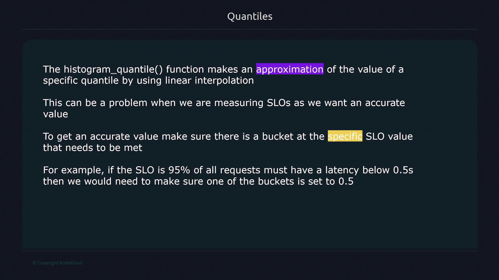
Histogram metrics can also help you compute quantiles (percentiles) using the histogram_quantile function. Quantiles indicate the value below which a specific percentage of data falls. For instance, to calculate the 75th percentile (indicating that 75% of data falls below a threshold), use:

$ histogram_quantile(0.75, request_latency_seconds_bucket)

An example output might be:

{instance="192.168.1.66:8000", job="api", method="GET", path="/articles"} 0.076

This output informs us that 75% of requests had a latency of 0.076 seconds or less.

Similarly, to verify if a Service Level Objective (SLO) is met—such as 95% of requests completing in under 0.5 seconds—execute:

$ histogram_quantile(0.95, request_latency_seconds_bucket)

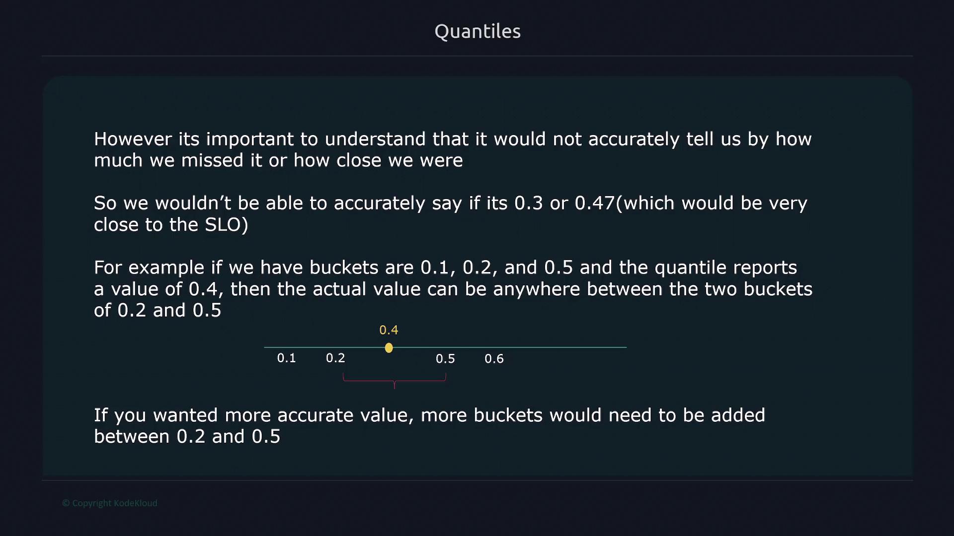
If the result exceeds 0.5, the SLO is not being met. Remember that the histogram_quantile function approximates the quantile using linear interpolation between bucket values. To enhance accuracy, include a bucket that matches your SLO limit. For instance, if your SLO is 0.5 seconds, ensure a bucket is defined for that value.

Below is an image that illustrates the linear interpolation method used in histogram_quantile(), emphasizing the need for a bucket at the SLO value:

Another image below demonstrates the accuracy limitations inherent to bucketed values and suggests that more buckets can lead to better quantile approximation:

Prometheus Web Interface and Metric Subcomponents

Understanding the breakdown of a typical request latency histogram in Prometheus is essential. A histogram metric is broken down into three main components:

• Buckets: Detailed breakdown of request counts per defined latency bucket.
• Count: Total number of processed requests.
• Sum: Accumulated request latency sum.

For example, here’s how the count metric might appear:

request_latency_seconds_count{instance="192.168.1.168:8000", job="api", method="GET"}

And for the sum metric:

request_latency_seconds_sum{instance="192.168.1.168:8000", job="api", method="GET"}

If every request consistently took one second, the sum would equal 100 seconds for 100 requests. In practice, if the sum is 50 seconds, it indicates that request latencies vary.

The bucket metrics provide additional granularity. For a specific request path (for example, /cars), you might observe:

request_latency_seconds_bucket{instance="192.168.1.168:8000", job="api", le="0.01", method="/cars", path="GET"}
request_latency_seconds_bucket{instance="192.168.1.168:8000", job="api", le="0.02", method="/cars", path="GET"}
request_latency_seconds_bucket{instance="192.168.1.168:8000", job="api", le="0.04", method="/cars", path="GET"}
request_latency_seconds_bucket{instance="192.168.1.168:8000", job="api", le="0.05", method="/cars", path="GET"}
request_latency_seconds_bucket{instance="192.168.1.168:8000", job="api", le="0.1", method="/cars", path="GET"}
request_latency_seconds_bucket{instance="192.168.1.168:8000", job="api", le="0.2", method="/cars", path="GET"}
request_latency_seconds_bucket{instance="192.168.1.168:8000", job="api", le="0.3", method="/cars", path="GET"}
request_latency_seconds_bucket{instance="192.168.1.168:8000", job="api", le="0.6", method="/cars", path="GET"}
request_latency_seconds_bucket{instance="192.168.1.168:8000", job="api", le="1.0", method="/cars", path="GET"}
request_latency_seconds_bucket{instance="192.168.1.168:8000", job="api", le="1.5", method="/cars", path="GET"}
request_latency_seconds_bucket{instance="192.168.1.168:8000", job="api", le="2.0", method="/cars", path="GET"}
request_latency_seconds_bucket{instance="192.168.1.168:8000", job="api", le="3.0", method="/cars", path="GET"}
request_latency_seconds_bucket{instance="192.168.1.168:8000", job="api", le="5.0", method="/cars", path="GET"}
request_latency_seconds_bucket{instance="192.168.1.168:8000", job="api", le="10.0", method="/cars", path="GET"}
request_latency_seconds_bucket{instance="192.168.1.168:8000", job="api", le="100.0", method="/cars", path="GET"}

A sample cumulative breakdown might look like this:

request_latency_seconds_bucket{instance="192.168.1.168:8000", job="api", le="0.01", method="/cars", path="GET"} 100
request_latency_seconds_bucket{instance="192.168.1.168:8000", job="api", le="0.02", method="/cars", path="GET"} 2
request_latency_seconds_bucket{instance="192.168.1.168:8000", job="api", le="0.03", method="/cars", path="GET"} 3
request_latency_seconds_bucket{instance="192.168.1.168:8000", job="api", le="0.05", method="/cars", path="GET"} 5
request_latency_seconds_bucket{instance="192.168.1.168:8000", job="api", le="0.1", method="/cars", path="GET"} 6
request_latency_seconds_bucket{instance="192.168.1.168:8000", job="api", le="0.2", method="/cars", path="GET"} 10
request_latency_seconds_bucket{instance="192.168.1.168:8000", job="api", le="0.3", method="/cars", path="GET"} 14
request_latency_seconds_bucket{instance="192.168.1.168:8000", job="api", le="0.4", method="/cars", path="GET"} 15
request_latency_seconds_bucket{instance="192.168.1.168:8000", job="api", le="0.5", method="/cars", path="GET"} 18
request_latency_seconds_bucket{instance="192.168.1.168:8000", job="api", le="1", method="/cars", path="GET"} 31
request_latency_seconds_bucket{instance="192.168.1.168:8000", job="api", le="2", method="/cars", path="GET"} 57
request_latency_seconds_bucket{instance="192.168.1.168:8000", job="api", le="5", method="/cars", path="GET"} 89
request_latency_seconds_bucket{instance="192.168.1.168:8000", job="api", le="10", method="/cars", path="GET"} 99
request_latency_seconds_bucket{instance="192.168.1.168:8000", job="api", le="+Inf", method="/cars", path="GET"} 100

Below is an image showing the Prometheus web interface and how you can query available metrics for request latency:

Calculating a Quantile Example

To calculate the 95th percentile for request latency of your API, use the histogram_quantile function. This query returns the latency value below which 95% of requests fall:

histogram_quantile(0.95, request_latency_seconds_bucket{instance="192.168.1.168:8000", job="api", method="GET"})

The query output is:

0.96

This result means that 95% of the requests completed with a latency of 0.96 seconds or less.

Summary Metrics: An Alternative Approach

Summary metrics operate similarly to histograms but expose precomputed quantiles directly. They consist of:

• Count: Total number of samples.
• Sum: Total sum of all sample values.
• Precomputed Quantiles: Each quantile is directly available as a sub-metric with its corresponding label.

An example of a summary metric is shown below:

request_latency_seconds_count{path="/articles"} 100
request_latency_seconds_sum{path="/articles"} 3.144

Where instead of calculating quantiles from buckets, the summary metric already includes quantiles (e.g., a quantile of 0.7 indicating 70% of requests had a latency below 0.0365 seconds). Note that with summaries, quantiles must be predefined in your instrumentation code.

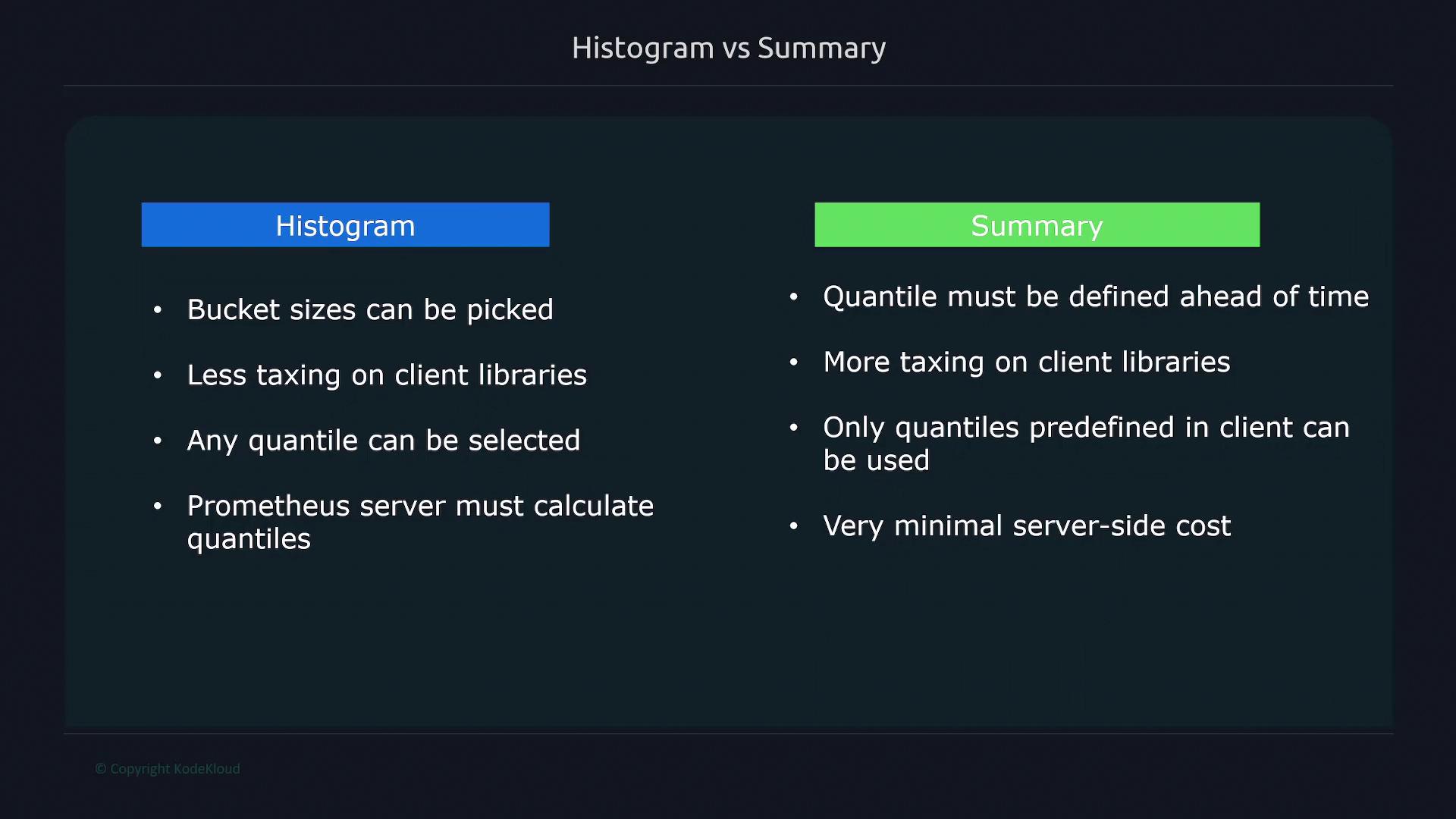
Comparison: Histograms vs. Summaries

Choose the metric type that best aligns with your monitoring needs and infrastructure constraints.

Below is an image that visually compares histograms and summaries, highlighting bucket sizing, client impact, quantile selection, and associated server overhead:

In summary, histograms provide flexibility by allowing any quantile to be calculated at query time using linear interpolation, whereas summaries offer the convenience of precomputed quantiles with reduced load on the server. Select the approach that best suits your specific use case.

Happy monitoring!