> ## Documentation Index
> Fetch the complete documentation index at: https://notes.kodekloud.com/llms.txt
> Use this file to discover all available pages before exploring further.
# HNSW Construction and Adoption
> Guide to constructing and tuning HNSW graphs for vector search, detailing insertion, layer assignment, neighbor selection, and key parameters M efConstruction and ef for performance trade-offs
Hello and welcome back.
Now that HNSW is understood as a multi-layer graph, this guide shows how to build and use it in practice. We walk through how a new vector is inserted and how the structure is tuned for performance.
Insertion into HNSW is a multi-step process:
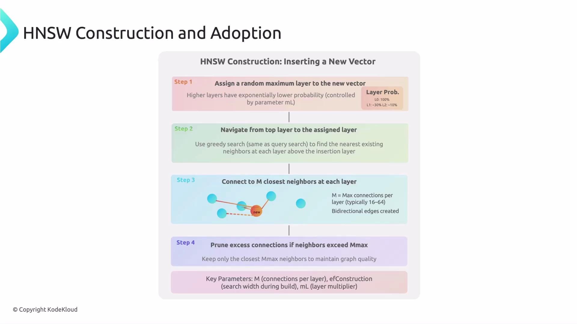
1. Assign a random maximum layer to the new vector\
Each new element is assigned a random maximum layer. Higher layers are exponentially rarer than lower ones, producing a pyramid-like topology: only a small subset of vectors appear in top layers while most vectors remain near the base. This sparsity at higher layers keeps long-range routing efficient. The distribution is controlled by a level-distribution parameter (often tied to `M` and implementation defaults).
2. Navigate from the top layer down to the target layer\
Insertion starts from a global entry point (typically a node located in the top layer). At each layer, the algorithm performs a greedy search: move to the neighbor that is closer to the new vector repeatedly until reaching a local minimum (no neighbor is closer). That local minimum becomes the entry point for the next lower layer. Repeat this until you reach the layer where the new vector will be inserted.
3. Connect the new vector to its neighbors\
For every layer where the new vector should appear, HNSW performs a best-first search (candidate list size determined by `efConstruction`) to find the best neighbor candidates. The algorithm then connects the new node to up to `M` nearest neighbors at that layer. Connections are bidirectional—if A connects to B, B also links back to A—ensuring bidirectional navigability.
4. Prune and select neighbors (diversification)\
If connecting the new node would exceed a node’s `M` limit, a neighbor-selection heuristic prunes connections to keep the closest and most diversifying neighbors. This diversification preserves search quality while preventing layers from becoming overly dense.
Key parameters that control HNSW behavior
 | Parameter | What it controls | Typical effect / guidance |
| ----------------- | ---------------------------------------------------- | -------------------------------------------------------------------------------------------------------------------------------- |
| `M` | Maximum number of connections per node at each layer | Higher `M` → better connectivity and recall but more memory and maintenance overhead. Common defaults: `16` or `32`. |
| `efConstruction` | Candidate list size during index construction | Larger `efConstruction` → better-connected index and higher recall, at the cost of slower indexing and more memory during build. |
| `ef` / `efSearch` | Candidate list size during queries | Larger `ef` → higher recall at query time, but with increased query latency. Tune to the desired recall/latency balance. |
Tuning notes:
* Increase `efConstruction` and/or `M` to improve index quality (higher recall) — expect longer build times and greater memory use.
* Increase query `ef` to improve accuracy at query time — expect longer queries.
* Typical production strategy: tune `efConstruction` and `M` once (at index build time), then adjust `ef` dynamically per-query to meet latency/recall requirements.
Tune `efConstruction` to prioritize index-build quality and tune `ef` at query time to meet your recall versus latency goals. Higher values improve recall but consume more resources.
Why HNSW is popular
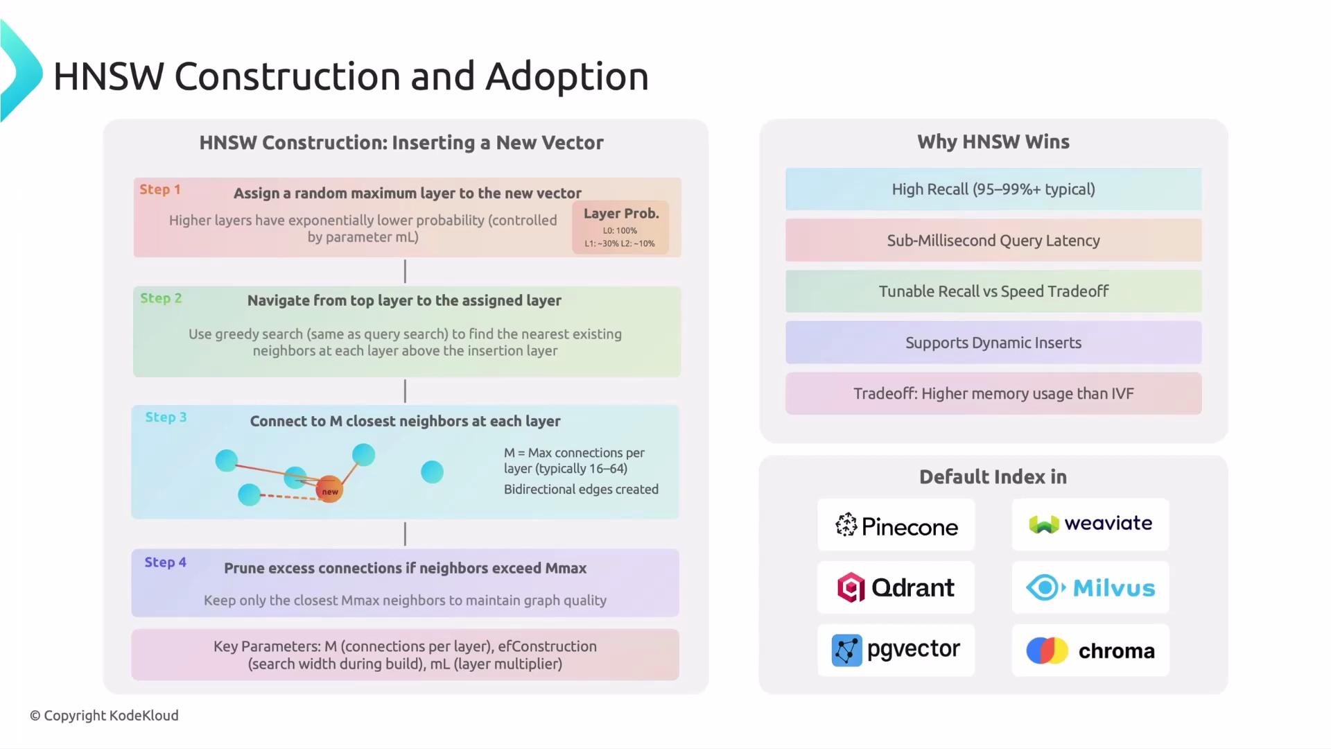
* High recall: HNSW often achieves very high recall (commonly in the mid-90s to high-90s percentiles), approximating true nearest neighbors closely.
* Very fast queries: On modern hardware, many queries run in sub-millisecond to single-digit-millisecond ranges, making HNSW suitable for real-time applications.
* Tunable trade-offs: `M`, `efConstruction`, and `ef` let you balance accuracy, build time, memory, and query latency.
* Broad ecosystem adoption: Many vector databases and libraries use HNSW as a default or recommended index (for example, [Pinecone](https://www.pinecone.io/), [Weaviate](https://weaviate.io/), [Qdrant](https://qdrant.tech/)). If you use production semantic search or recommendation systems, they’re likely powered by HNSW or a variant.
The trade-off: HNSW stores explicit links between vectors, so it typically requires more memory than simpler approximations (for example, inverted-file or PQ-based methods). In many applications the extra memory cost is justified by the speed and accuracy gains.
| Parameter | What it controls | Typical effect / guidance |
| ----------------- | ---------------------------------------------------- | -------------------------------------------------------------------------------------------------------------------------------- |
| `M` | Maximum number of connections per node at each layer | Higher `M` → better connectivity and recall but more memory and maintenance overhead. Common defaults: `16` or `32`. |
| `efConstruction` | Candidate list size during index construction | Larger `efConstruction` → better-connected index and higher recall, at the cost of slower indexing and more memory during build. |
| `ef` / `efSearch` | Candidate list size during queries | Larger `ef` → higher recall at query time, but with increased query latency. Tune to the desired recall/latency balance. |
Tuning notes:
* Increase `efConstruction` and/or `M` to improve index quality (higher recall) — expect longer build times and greater memory use.
* Increase query `ef` to improve accuracy at query time — expect longer queries.
* Typical production strategy: tune `efConstruction` and `M` once (at index build time), then adjust `ef` dynamically per-query to meet latency/recall requirements.
Tune `efConstruction` to prioritize index-build quality and tune `ef` at query time to meet your recall versus latency goals. Higher values improve recall but consume more resources.
Why HNSW is popular
* High recall: HNSW often achieves very high recall (commonly in the mid-90s to high-90s percentiles), approximating true nearest neighbors closely.
* Very fast queries: On modern hardware, many queries run in sub-millisecond to single-digit-millisecond ranges, making HNSW suitable for real-time applications.
* Tunable trade-offs: `M`, `efConstruction`, and `ef` let you balance accuracy, build time, memory, and query latency.
* Broad ecosystem adoption: Many vector databases and libraries use HNSW as a default or recommended index (for example, [Pinecone](https://www.pinecone.io/), [Weaviate](https://weaviate.io/), [Qdrant](https://qdrant.tech/)). If you use production semantic search or recommendation systems, they’re likely powered by HNSW or a variant.
The trade-off: HNSW stores explicit links between vectors, so it typically requires more memory than simpler approximations (for example, inverted-file or PQ-based methods). In many applications the extra memory cost is justified by the speed and accuracy gains.
 Summary
HNSW construction centers on four ideas:
1. Assign elements to exponentially distributed layers.
2. Navigate from a top-level entry point down using greedy search.
3. Connect new elements to up to `M` neighbors per layer using a best-first search sized by `efConstruction`.
4. Prune neighbors to preserve diversity and sparsity.
Properly tuning `M`, `efConstruction`, and `ef` lets you trade recall, indexing cost, memory, and query latency—making HNSW a practical default for production vector search.
That concludes the HNSW construction and adoption overview.
Summary
HNSW construction centers on four ideas:
1. Assign elements to exponentially distributed layers.
2. Navigate from a top-level entry point down using greedy search.
3. Connect new elements to up to `M` neighbors per layer using a best-first search sized by `efConstruction`.
4. Prune neighbors to preserve diversity and sparsity.
Properly tuning `M`, `efConstruction`, and `ef` lets you trade recall, indexing cost, memory, and query latency—making HNSW a practical default for production vector search.
That concludes the HNSW construction and adoption overview.