> ## Documentation Index
> Fetch the complete documentation index at: https://notes.kodekloud.com/llms.txt
> Use this file to discover all available pages before exploring further.
# HNSW Multi Layered Graph Structure
> Explains HNSW multi-layered graph index for fast approximate nearest neighbor search in vector databases, covering intuition, search workflow, parameters, and practical tuning.
Welcome back. This lesson explains HNSW (Hierarchical Navigable Small World), a multi-layered graph index commonly used inside vector databases to enable fast approximate nearest neighbor (ANN) search.
Why it matters: graph-based indexes like HNSW are the backbone of high-performance vector search. They let systems find similar vectors at scale with low latency while trading off a controlled amount of accuracy. This guide covers the intuition, the search workflow, and practical tuning considerations for HNSW.
What is HNSW (intuition)
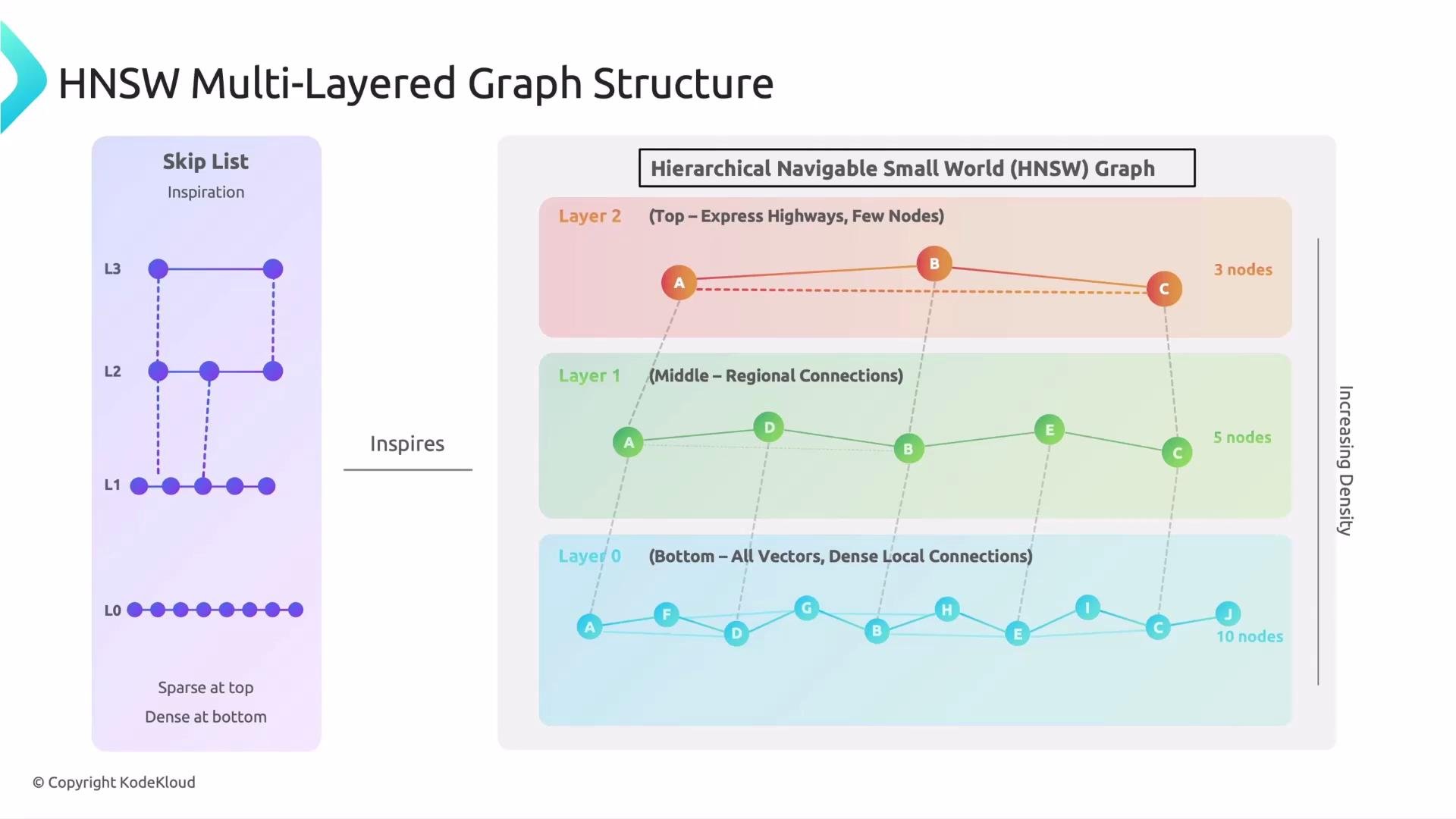
* HNSW is conceptually similar to a skip list: a hierarchy of layers where upper layers are sparse and lower layers are increasingly dense.
* Upper layers provide long-range shortcuts for coarse navigation across the embedding space.
* The bottom layer (level 0) contains all vectors and dense local links for precise nearest-neighbor retrieval.
At a glance:
* Top layers: very sparse, long-range links — fast coarse jumps.
* Middle layers: intermediate connectivity — guide search toward the target region.
* Bottom layer: dense connectivity with all points — final fine-grained search.
 How HNSW navigates search space
* Entry points at the top layer let you quickly traverse large distances in vector space.
* Each lower layer adds more nodes and more local edges, increasing search accuracy as you descend.
* The algorithm transitions from coarse to fine search: greedy climbs on sparse layers, and a more exhaustive candidate expansion on the bottom layer.
Search workflow (high-level)
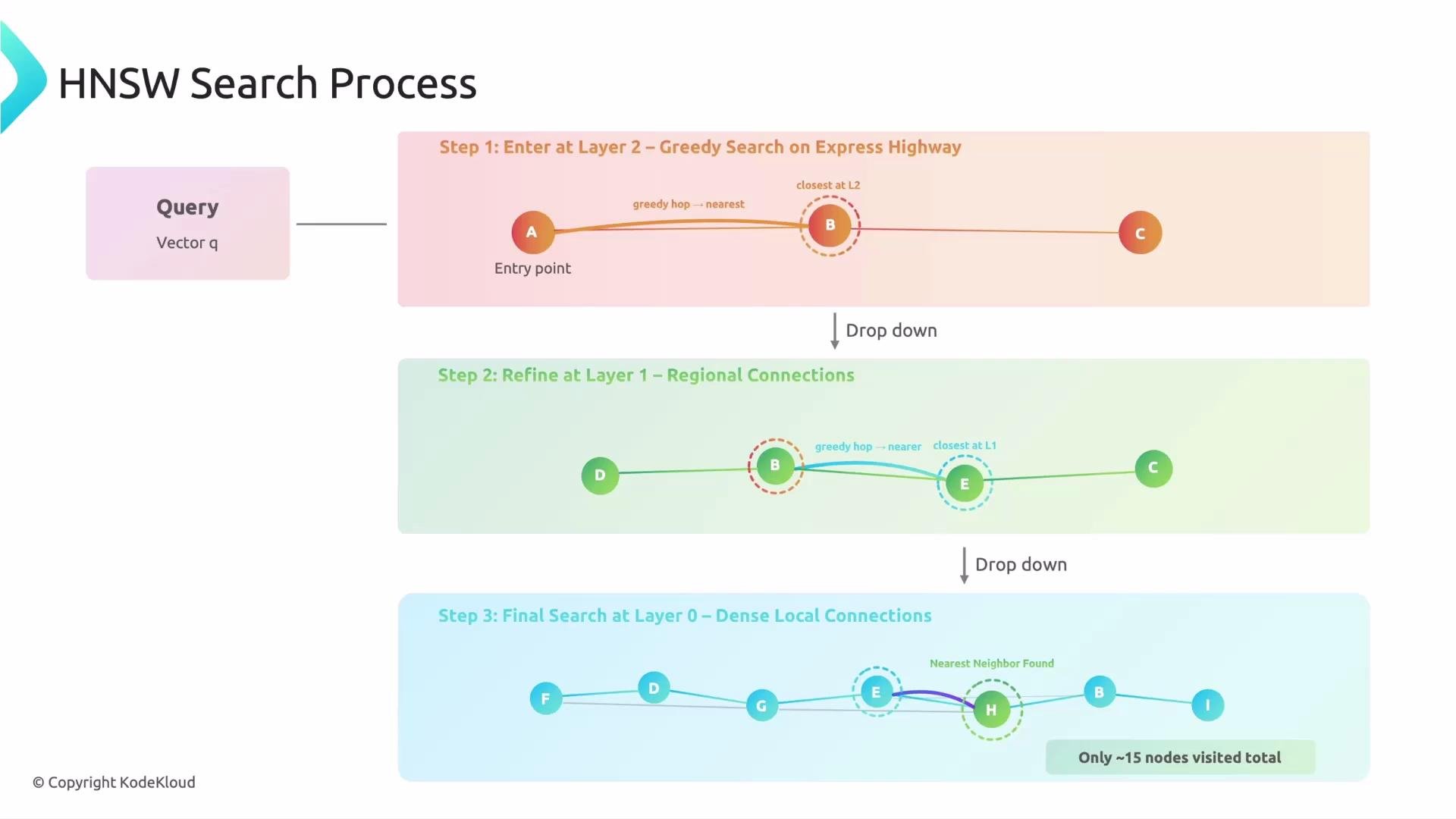
1. Provide a query vector and start from an entry point at the highest layer.
2. At each upper layer, perform greedy hill-climbing: repeatedly move to the neighbor that reduces distance to the query until no neighbor is closer. The goal is coarse localization.
3. Take the best point found in the current layer as the entry point into the next (denser) layer.
4. Repeat the greedy descent until reaching level 0 (the bottom layer).
5. At level 0, perform a best-first (priority queue) search controlled by `ef` (often called `efSearch`) to collect the final k nearest neighbors.
Pseudocode (simplified)
```text theme={null}
# Simplified HNSW query outline
entry = graph.top_entry_point
for level in descending_layers:
entry = greedy_search(entry, query_vector, level)
# At level 0:
result = best_first_search(entry, query_vector, efSearch, k)
return result
```
The greedy steps are fast because nodes have few links in upper layers and you only follow links that improve distance. The bottom layer’s best-first search explores a candidate set and balances recall vs latency via `efSearch`.
How HNSW navigates search space
* Entry points at the top layer let you quickly traverse large distances in vector space.
* Each lower layer adds more nodes and more local edges, increasing search accuracy as you descend.
* The algorithm transitions from coarse to fine search: greedy climbs on sparse layers, and a more exhaustive candidate expansion on the bottom layer.
Search workflow (high-level)
1. Provide a query vector and start from an entry point at the highest layer.
2. At each upper layer, perform greedy hill-climbing: repeatedly move to the neighbor that reduces distance to the query until no neighbor is closer. The goal is coarse localization.
3. Take the best point found in the current layer as the entry point into the next (denser) layer.
4. Repeat the greedy descent until reaching level 0 (the bottom layer).
5. At level 0, perform a best-first (priority queue) search controlled by `ef` (often called `efSearch`) to collect the final k nearest neighbors.
Pseudocode (simplified)
```text theme={null}
# Simplified HNSW query outline
entry = graph.top_entry_point
for level in descending_layers:
entry = greedy_search(entry, query_vector, level)
# At level 0:
result = best_first_search(entry, query_vector, efSearch, k)
return result
```
The greedy steps are fast because nodes have few links in upper layers and you only follow links that improve distance. The bottom layer’s best-first search explores a candidate set and balances recall vs latency via `efSearch`.
 Key parameters and their effects
| Parameter | Purpose | Typical effect / tuning guideline |
| ---------------------------------: | ------------------------------------------------------------ | --------------------------------------------------------------------------------- |
| `M` | Max connections per node (graph degree) | Higher `M` → better recall and connectivity, more memory and slower construction. |
| `efConstruction` | Size of the dynamic candidate list during index build | Larger → higher-quality index, longer build times and more memory. |
| `efSearch` | Size of the candidate list at query time (often called `ef`) | Larger → higher recall at query time, increased latency and CPU per query. |
| `level_mult` (or level generation) | Controls how many layers a node appears in | Affects height distribution and average search hops from top to bottom. |
HNSW is an approximate nearest neighbor algorithm. The most commonly tuned values are `M`, `efConstruction`, and `efSearch`. Adjust these to balance recall, query latency, and memory. For production, benchmark recall vs latency for representative queries and vectors.
Practical considerations and best practices
* Index construction: increase `efConstruction` and `M` if you need higher recall, especially for large or highly clustered datasets. Expect longer build times and higher memory use.
* Query tuning: raise `efSearch` to improve recall for difficult queries; lower it to reduce latency when recall requirements are modest.
* Memory vs performance: higher connectivity (`M`) and larger dynamic lists require more memory. Monitor memory consumption on nodes that host the index.
* Entry point strategy: most implementations pick a randomized or high-degree node as entry. Consistent entry strategies help with predictable latency.
* Parallelism: many HNSW libs support parallel index building and multi-threaded searching — use available cores carefully for a production workload.
Real-world example
Imagine an e-commerce recommendation engine. When a user views a product, the system uses HNSW instead of comparing the current product vector to every catalog item. The index quickly jumps to the correct product region (e.g., shirts, electronics), then refines within that local neighborhood to return relevant recommendations in milliseconds. This is how features like “customers who bought this also bought” are generated in near real time.
References and further reading
* Malkov, Y. A., & Yashunin, D. A. (2018). Efficient and robust approximate nearest neighbor search using Hierarchical Navigable Small World graphs (HNSW). [Original HNSW paper](https://arxiv.org/abs/1603.09320)
* [Faiss — Facebook AI Similarity Search](https://github.com/facebookresearch/faiss)
* [nmslib — Similarity Search library](https://github.com/nmslib/nmslib)
Next lessons will cover how HNSW integrates inside vector databases (index construction patterns, distributed deployments, and tuning strategies for production). Thanks for reading.
Key parameters and their effects
| Parameter | Purpose | Typical effect / tuning guideline |
| ---------------------------------: | ------------------------------------------------------------ | --------------------------------------------------------------------------------- |
| `M` | Max connections per node (graph degree) | Higher `M` → better recall and connectivity, more memory and slower construction. |
| `efConstruction` | Size of the dynamic candidate list during index build | Larger → higher-quality index, longer build times and more memory. |
| `efSearch` | Size of the candidate list at query time (often called `ef`) | Larger → higher recall at query time, increased latency and CPU per query. |
| `level_mult` (or level generation) | Controls how many layers a node appears in | Affects height distribution and average search hops from top to bottom. |
HNSW is an approximate nearest neighbor algorithm. The most commonly tuned values are `M`, `efConstruction`, and `efSearch`. Adjust these to balance recall, query latency, and memory. For production, benchmark recall vs latency for representative queries and vectors.
Practical considerations and best practices
* Index construction: increase `efConstruction` and `M` if you need higher recall, especially for large or highly clustered datasets. Expect longer build times and higher memory use.
* Query tuning: raise `efSearch` to improve recall for difficult queries; lower it to reduce latency when recall requirements are modest.
* Memory vs performance: higher connectivity (`M`) and larger dynamic lists require more memory. Monitor memory consumption on nodes that host the index.
* Entry point strategy: most implementations pick a randomized or high-degree node as entry. Consistent entry strategies help with predictable latency.
* Parallelism: many HNSW libs support parallel index building and multi-threaded searching — use available cores carefully for a production workload.
Real-world example
Imagine an e-commerce recommendation engine. When a user views a product, the system uses HNSW instead of comparing the current product vector to every catalog item. The index quickly jumps to the correct product region (e.g., shirts, electronics), then refines within that local neighborhood to return relevant recommendations in milliseconds. This is how features like “customers who bought this also bought” are generated in near real time.
References and further reading
* Malkov, Y. A., & Yashunin, D. A. (2018). Efficient and robust approximate nearest neighbor search using Hierarchical Navigable Small World graphs (HNSW). [Original HNSW paper](https://arxiv.org/abs/1603.09320)
* [Faiss — Facebook AI Similarity Search](https://github.com/facebookresearch/faiss)
* [nmslib — Similarity Search library](https://github.com/nmslib/nmslib)
Next lessons will cover how HNSW integrates inside vector databases (index construction patterns, distributed deployments, and tuning strategies for production). Thanks for reading.