> ## Documentation Index
> Fetch the complete documentation index at: https://notes.kodekloud.com/llms.txt
> Use this file to discover all available pages before exploring further.
# Indexing in Vector Database
> Explains why brute force vector search fails at scale and how ANN indexing techniques like graph, hashing, trees, and quantization enable efficient, scalable nearest neighbor search with trade offs
Hello and welcome back.
What if the way most people imagine vector search actually falls apart the moment you try to use it in production? This lesson explains why a naive approach doesn't scale, how indexing fixes it, and which indexing strategies are commonly used in real-world systems.
## Brute-force (linear scan)
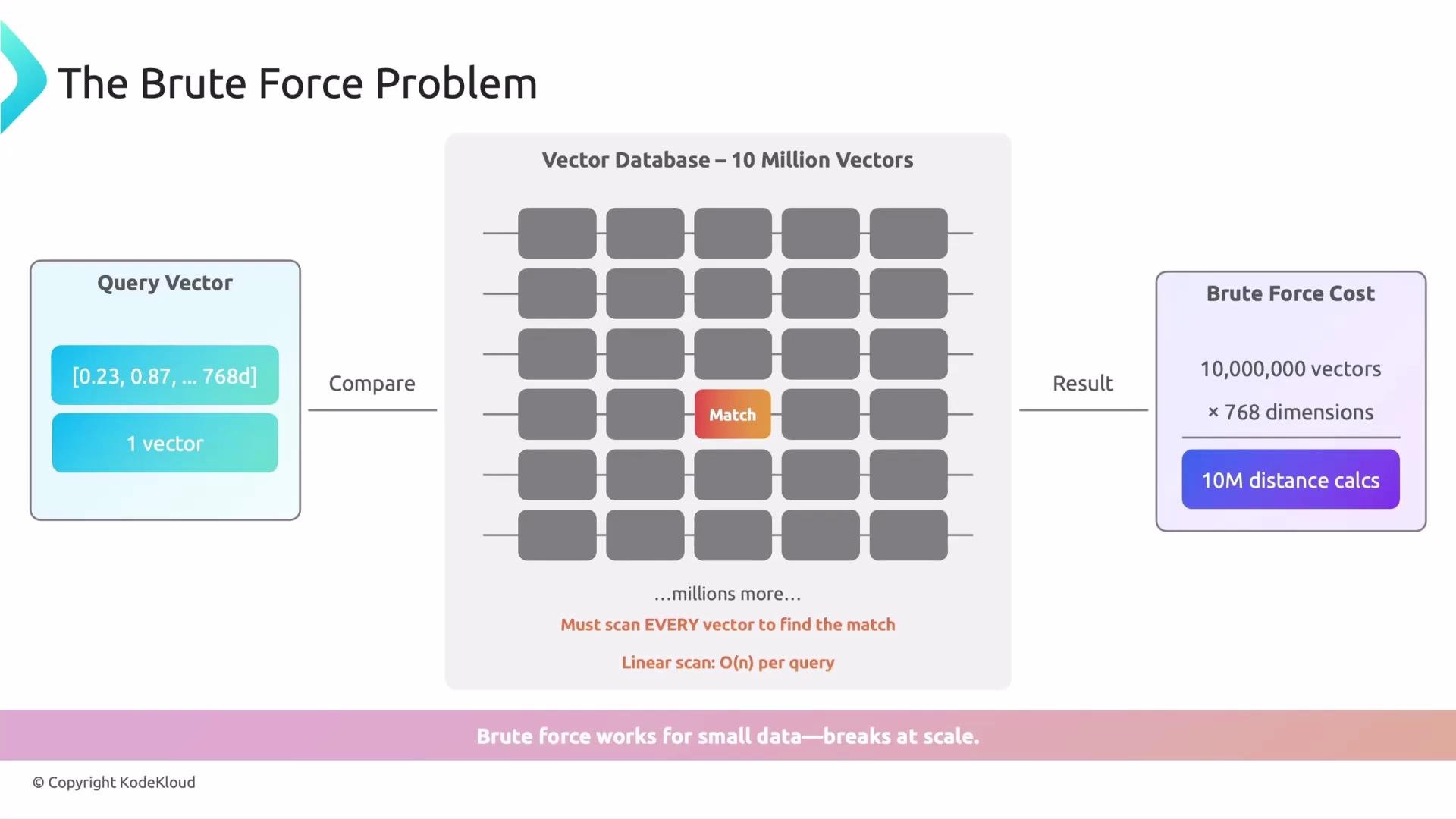
Brute force, or a linear scan, is the simplest way to run a nearest-neighbor search:
* You submit a query vector (for example, `[0.23, 0.87, ...]` in 768 dimensions).
* The system compares that query against every vector stored in the database.
* If the database contains 10 million vectors, the system makes 10 million distance calculations per query, one-by-one, to find the closest matches.
Think of it as trying to find a friend in a stadium by shaking hands with every single person until you find them. It works, but it’s painfully slow and unscalable: cost grows linearly with dataset size.
Practical cost: each query with N vectors and D dimensions requires roughly O(N × D) distance computations. For large-scale applications—Pinterest-style visual similarity, recommendation systems, or large document corpora—brute force rapidly becomes infeasible.
Brute force is fine for small datasets; it breaks at scale.
 ## Indexing to the rescue
Indexing is the set of techniques that let you avoid examining every vector. A simple analogy is a library:
* Without an index, you open every book on every shelf until you find the one you want (linear scan).
* With an index (catalog), you look up the catalog, go to the right section, and search only a small subset of books.
In vector search, indexes are data structures and algorithms for nearest neighbor search that let you skip irrelevant regions of the vector space and inspect only a small subset of candidates. Instead of checking all 10 million vectors, an index might reduce the candidates to a few thousand—or a few hundred—dramatically lowering CPU and memory costs.
Indexing typically uses Approximate Nearest Neighbor (ANN) techniques to deliver sublinear query latencies in large vector collections. This commonly trades a tiny amount of recall for orders-of-magnitude improvements in throughput and cost.
## Complexity and trade-offs
* Linear scan: typically O(N × D) per query.
* Index-based search: can achieve sublinear behavior in N for many workloads; some structures aim for \~O(log N) under ideal conditions, but real-world performance depends on the algorithm, implementation, and data dimensionality.
High dimensionality can degrade index effectiveness and increase false negatives; choosing the right index is a trade-off among recall, latency, memory footprint, build time, and update cost.
High dimensional vectors (very large D) can reduce the effectiveness of many indexes. Always benchmark with your data distribution and query patterns—synthetic tests can be misleading.
## Common ANN approaches
Here’s a concise comparison of standard ANN techniques and where they shine:
| Approach | Best for | Pros | Cons | Examples / Notes |
| --------------------- | ------------------------------------------- | ------------------------------------------------------------------------ | --------------------------------------------- | ----------------------------------------- |
| Tree-based | Low to moderate dimensions | Intuitive, good exact or near-exact performance in small D | Degrades as D grows | KD-trees, randomized trees |
| Hashing (LSH) | Sublinear lookup under specific distances | Fast lookup via buckets, good for particular distance functions | Parameter tuning; limited distance metrics | Locality-Sensitive Hashing (LSH) |
| Graph-based indices | General high-performance ANN | Excellent empirical speed/accuracy balance; efficient neighbor traversal | Memory overhead, more complex to build/update | HNSW (Hierarchical Navigable Small World) |
| Quantization / IVF+PQ | Very large collections where memory matters | Huge memory savings, faster distance computation | Some accuracy loss; complex hybrid setups | Product Quantization (PQ), IVF+PQ |
For more in-depth reading:
* [HNSW paper and implementations](https://arxiv.org/abs/1603.09320)
* [Overview of Product Quantization](https://arxiv.org/abs/1106.1968)
* [Locality-Sensitive Hashing (LSH) concepts](https://en.wikipedia.org/wiki/Locality-sensitive_hashing)
## Practical guidelines
* Start with a baseline: measure brute-force latency and recall to understand performance targets.
* Profile your data: dimensionality, sparsity, and cluster structure affect index choice.
* Benchmark multiple index types using realistic query loads and realistic candidate set sizes.
* Consider hybrid approaches: graph indices combined with quantization or inverted lists scale well in production.
* Monitor recall/precision trade-offs: tune index parameters (e.g., number of probes, ef/search size) to meet application SLAs.
## Summary
* Brute force performs a full linear scan and becomes impractical as N grows.
* Indexing provides a catalog-like shortcut to inspect only a small region of relevant vectors.
* ANN indexes (graph-based, hashing, trees, quantization) are the practical solution for scalable vector search. Each offers trade-offs between speed, memory, build time, and accuracy—benchmark with your real data.
That’s it for this lesson. See you in the next lesson.
## Links and References
* [KNN and ANN fundamentals (survey)](https://en.wikipedia.org/wiki/K-nearest_neighbors_algorithm)
* [HNSW (Graph-based ANN)](https://github.com/nmslib/hnswlib)
* [FAISS — Facebook AI Similarity Search](https://github.com/facebookresearch/faiss)
## Indexing to the rescue
Indexing is the set of techniques that let you avoid examining every vector. A simple analogy is a library:
* Without an index, you open every book on every shelf until you find the one you want (linear scan).
* With an index (catalog), you look up the catalog, go to the right section, and search only a small subset of books.
In vector search, indexes are data structures and algorithms for nearest neighbor search that let you skip irrelevant regions of the vector space and inspect only a small subset of candidates. Instead of checking all 10 million vectors, an index might reduce the candidates to a few thousand—or a few hundred—dramatically lowering CPU and memory costs.
Indexing typically uses Approximate Nearest Neighbor (ANN) techniques to deliver sublinear query latencies in large vector collections. This commonly trades a tiny amount of recall for orders-of-magnitude improvements in throughput and cost.
## Complexity and trade-offs
* Linear scan: typically O(N × D) per query.
* Index-based search: can achieve sublinear behavior in N for many workloads; some structures aim for \~O(log N) under ideal conditions, but real-world performance depends on the algorithm, implementation, and data dimensionality.
High dimensionality can degrade index effectiveness and increase false negatives; choosing the right index is a trade-off among recall, latency, memory footprint, build time, and update cost.
High dimensional vectors (very large D) can reduce the effectiveness of many indexes. Always benchmark with your data distribution and query patterns—synthetic tests can be misleading.
## Common ANN approaches
Here’s a concise comparison of standard ANN techniques and where they shine:
| Approach | Best for | Pros | Cons | Examples / Notes |
| --------------------- | ------------------------------------------- | ------------------------------------------------------------------------ | --------------------------------------------- | ----------------------------------------- |
| Tree-based | Low to moderate dimensions | Intuitive, good exact or near-exact performance in small D | Degrades as D grows | KD-trees, randomized trees |
| Hashing (LSH) | Sublinear lookup under specific distances | Fast lookup via buckets, good for particular distance functions | Parameter tuning; limited distance metrics | Locality-Sensitive Hashing (LSH) |
| Graph-based indices | General high-performance ANN | Excellent empirical speed/accuracy balance; efficient neighbor traversal | Memory overhead, more complex to build/update | HNSW (Hierarchical Navigable Small World) |
| Quantization / IVF+PQ | Very large collections where memory matters | Huge memory savings, faster distance computation | Some accuracy loss; complex hybrid setups | Product Quantization (PQ), IVF+PQ |
For more in-depth reading:
* [HNSW paper and implementations](https://arxiv.org/abs/1603.09320)
* [Overview of Product Quantization](https://arxiv.org/abs/1106.1968)
* [Locality-Sensitive Hashing (LSH) concepts](https://en.wikipedia.org/wiki/Locality-sensitive_hashing)
## Practical guidelines
* Start with a baseline: measure brute-force latency and recall to understand performance targets.
* Profile your data: dimensionality, sparsity, and cluster structure affect index choice.
* Benchmark multiple index types using realistic query loads and realistic candidate set sizes.
* Consider hybrid approaches: graph indices combined with quantization or inverted lists scale well in production.
* Monitor recall/precision trade-offs: tune index parameters (e.g., number of probes, ef/search size) to meet application SLAs.
## Summary
* Brute force performs a full linear scan and becomes impractical as N grows.
* Indexing provides a catalog-like shortcut to inspect only a small region of relevant vectors.
* ANN indexes (graph-based, hashing, trees, quantization) are the practical solution for scalable vector search. Each offers trade-offs between speed, memory, build time, and accuracy—benchmark with your real data.
That’s it for this lesson. See you in the next lesson.
## Links and References
* [KNN and ANN fundamentals (survey)](https://en.wikipedia.org/wiki/K-nearest_neighbors_algorithm)
* [HNSW (Graph-based ANN)](https://github.com/nmslib/hnswlib)
* [FAISS — Facebook AI Similarity Search](https://github.com/facebookresearch/faiss)