> ## Documentation Index
> Fetch the complete documentation index at: https://notes.kodekloud.com/llms.txt
> Use this file to discover all available pages before exploring further.
# Quantization
> Overview of quantization techniques for compressing embeddings in vector databases, comparing product, scalar, and binary methods, their tradeoffs, and guidance for balancing compression versus recall
Welcome back.
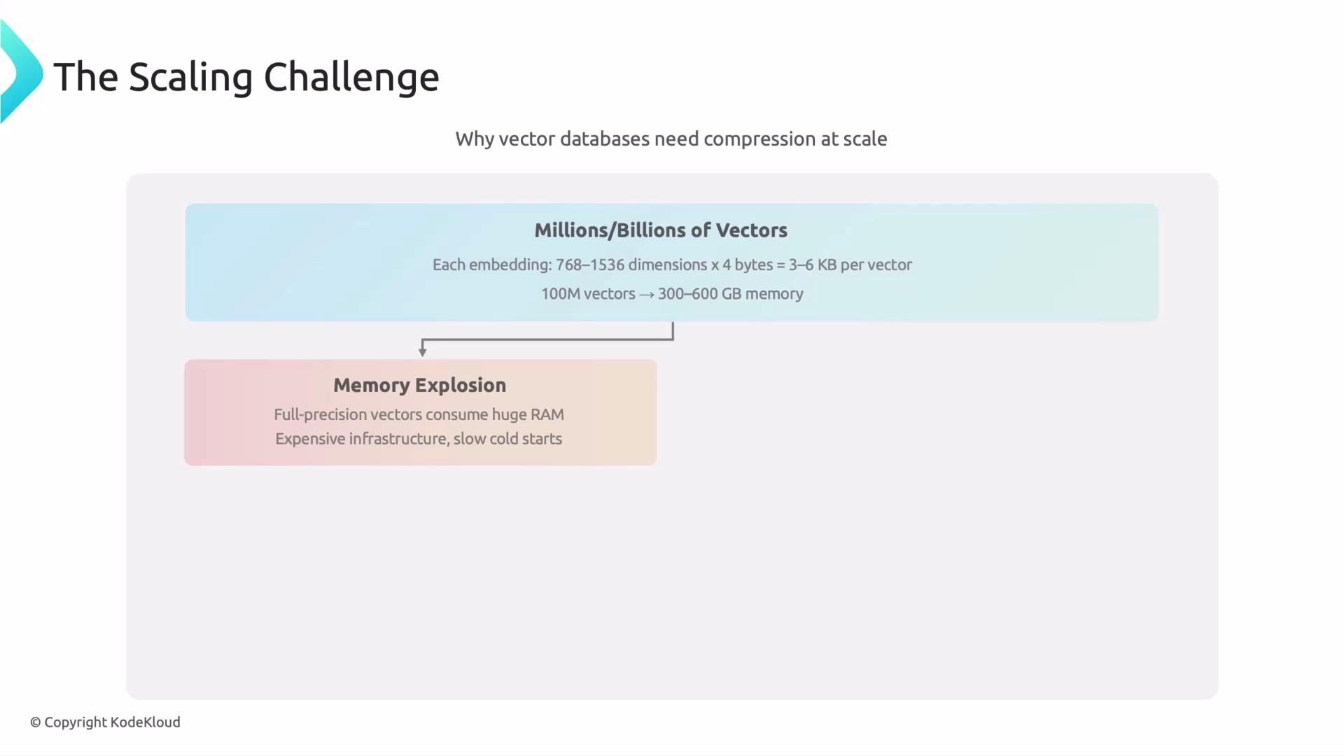
As embedding-driven systems move from prototype to production, they face a scaling problem: millions or billions of vectors, each often 768 or 1536 dimensions long, quickly consume RAM and increase search latency and cost. Typical embeddings are stored as 32-bit floats; for example:
```text theme={null}
1536 dimensions × 4 bytes = 6,144 bytes ≈ 6 KB per vector
```
At scale, this becomes prohibitive—100 million such vectors would need on the order of 600 GB of memory just to hold the raw vectors. That memory footprint increases startup time, operational cost, and the latency of nearest-neighbor search operations. To manage this, production systems use compression and approximation techniques under the umbrella term quantization.
 Think of a company like Spotify: comparing millions of user and track embeddings in full precision for every request would be infeasible. Quantization reduces storage per vector and speeds up distance computations by replacing full-precision vectors with compact representations.
This article overviews the major quantization families used in vector databases and ANN (Approximate Nearest Neighbor) search systems: product quantization, scalar quantization, and binary quantization.
## Main quantization techniques
| Method | What it does | Typical trade-offs |
| ------------------------------------- | ------------------------------------------------------------------------------------------------: | ------------------------------------------------------------------------------------------------------- |
| Product Quantization (PQ) | Splits vectors into sub-vectors and encodes each with an index into a small codebook (centroids). | Good balance of compression vs recall; enables fast asymmetric distance computation with lookup tables. |
| Scalar Quantization | Quantizes each scalar dimension independently (e.g., 8-bit per dimension). | Simple and fast; moderate compression (typically 2–4×) but can lose cross-dimension structure. |
| Binary Quantization (1-bit / Hashing) | Maps scalars to bits (sign or learned binary codes) and uses Hamming distance for search. | Extremely compact and fast; highest information loss and largest recall drop. |
### Product Quantization (PQ)
* Intuition: preserve cross-dimension structure by partitioning a D-dimensional vector into M sub-vectors and representing each sub-vector with a centroid index from a small codebook.
* How it works (high level):
1. Partition each D-dim vector into M sub-vectors of size D/M.
2. For each subspace, learn K centroids (k-means) → a codebook per subspace.
3. Encode each sub-vector as the index of its nearest centroid.
4. Store the vector as M small integers (one per subspace). Distance queries use precomputed lookup tables for asymmetric distance computation (ADC).
* Storage formula: storage per vector ≈ M × log2(K) bits. Example: if each code is one byte (K ≤ 256), storage ≈ M bytes.
* Benefits:
* Preserves part of the vector’s structure across dimensions.
* Often the best practical trade-off for large-scale ANN: substantial compression with reasonable recall.
* Enables fast distance computations with precomputed LUTs.
* Trade-offs:
* Reconstruction is approximate; choice of M and K controls accuracy vs storage.
* Codebook training (k-means) is an extra preprocessing cost.
### Scalar Quantization
* Intuition: compress each dimension independently by mapping float values to a discrete set of levels.
* How it works:
* Choose a bit depth per dimension (e.g., 8-bit), estimate range or per-dimension scale, and quantize each float32 to an integer bucket.
* Reconstruct by mapping integers back to approximate real values using the quantization step and offset.
* Benefits:
* Very simple and fast to apply.
* Predictable storage reduction: `float32 → uint8` gives \~4× savings.
* Works well when per-dimension variance is stable.
* Trade-offs:
* Ignores correlations among dimensions; can lose structure important for similarity.
* Requires appropriate range/scale selection or per-dimension calibration to avoid saturation.
### Binary Quantization (1-bit / Binary Hashing)
* Intuition: collapse values to bits—use the sign of projections or learn binary codes to represent vectors with minimal storage.
* How it works:
* Projection + sign: project vectors onto random or learned directions and take the sign (−1/+1 or 0/1).
* Learned binary codes: optimize bit assignments to preserve similarity in a supervised or unsupervised way.
* Use Hamming distance for very fast lookup.
* Benefits:
* Maximal compression (up to 32× vs float32 if using 1-bit per scalar).
* Extremely fast distance computations (bitwise XOR + population count).
* Trade-offs:
* Very aggressive; substantial loss of fine-grained information.
* Typically largest accuracy drop among quantization methods.
Quantization reduces memory footprint and speeds up search at the expense of approximation error. Choose the method and compression level that balance your application’s latency, throughput, and recall requirements.
## Choosing the right method
* Use Product Quantization when:
* You need significant compression with minimal loss of recall.
* You can afford codebook training and want fast ADC-style distance computation.
* Use Scalar Quantization when:
* You want a simple, predictable reduction in storage and fast encoding/decoding.
* Your vectors have stable per-dimension ranges or you apply per-dimension scaling.
* Use Binary Quantization when:
* Storage is extremely constrained or you need the absolute fastest Hamming-based search.
* You accept a larger drop in accuracy for extreme speed/compactness.
## Practical considerations and trade-offs
* Accuracy vs Storage: higher compression reduces recall. Tune parameters (e.g., M and K for PQ, bit-depth for scalar quantization) on a validation set to hit your SLA.
* Search latency: compressed representations often allow faster distance evaluations (lookup tables, bit operations) and better cache efficiency.
* Indexing and retrieval pipeline: combine quantization with ANN index structures (IVF, HNSW, etc.) for best overall performance.
* Training cost: PQ needs k-means per subspace; scalar quantization may require range estimation; binary methods may need supervised optimization.
References and further reading:
* [Approximate Nearest Neighbors (ANN)](https://en.wikipedia.org/wiki/Approximate_nearest_neighbor_search)
* [Product Quantization for Nearest Neighbor Search (original paper)](https://hal.inria.fr/inria-00548512/document)
* [HNSW: efficient ANN graph-based index](https://arxiv.org/abs/1603.09320)
That covers the basic ideas behind quantization and why it matters for vector databases. In follow-up sections we will examine implementation patterns, concrete parameter choices, and eval strategies for tuning recall vs storage.
Think of a company like Spotify: comparing millions of user and track embeddings in full precision for every request would be infeasible. Quantization reduces storage per vector and speeds up distance computations by replacing full-precision vectors with compact representations.
This article overviews the major quantization families used in vector databases and ANN (Approximate Nearest Neighbor) search systems: product quantization, scalar quantization, and binary quantization.
## Main quantization techniques
| Method | What it does | Typical trade-offs |
| ------------------------------------- | ------------------------------------------------------------------------------------------------: | ------------------------------------------------------------------------------------------------------- |
| Product Quantization (PQ) | Splits vectors into sub-vectors and encodes each with an index into a small codebook (centroids). | Good balance of compression vs recall; enables fast asymmetric distance computation with lookup tables. |
| Scalar Quantization | Quantizes each scalar dimension independently (e.g., 8-bit per dimension). | Simple and fast; moderate compression (typically 2–4×) but can lose cross-dimension structure. |
| Binary Quantization (1-bit / Hashing) | Maps scalars to bits (sign or learned binary codes) and uses Hamming distance for search. | Extremely compact and fast; highest information loss and largest recall drop. |
### Product Quantization (PQ)
* Intuition: preserve cross-dimension structure by partitioning a D-dimensional vector into M sub-vectors and representing each sub-vector with a centroid index from a small codebook.
* How it works (high level):
1. Partition each D-dim vector into M sub-vectors of size D/M.
2. For each subspace, learn K centroids (k-means) → a codebook per subspace.
3. Encode each sub-vector as the index of its nearest centroid.
4. Store the vector as M small integers (one per subspace). Distance queries use precomputed lookup tables for asymmetric distance computation (ADC).
* Storage formula: storage per vector ≈ M × log2(K) bits. Example: if each code is one byte (K ≤ 256), storage ≈ M bytes.
* Benefits:
* Preserves part of the vector’s structure across dimensions.
* Often the best practical trade-off for large-scale ANN: substantial compression with reasonable recall.
* Enables fast distance computations with precomputed LUTs.
* Trade-offs:
* Reconstruction is approximate; choice of M and K controls accuracy vs storage.
* Codebook training (k-means) is an extra preprocessing cost.
### Scalar Quantization
* Intuition: compress each dimension independently by mapping float values to a discrete set of levels.
* How it works:
* Choose a bit depth per dimension (e.g., 8-bit), estimate range or per-dimension scale, and quantize each float32 to an integer bucket.
* Reconstruct by mapping integers back to approximate real values using the quantization step and offset.
* Benefits:
* Very simple and fast to apply.
* Predictable storage reduction: `float32 → uint8` gives \~4× savings.
* Works well when per-dimension variance is stable.
* Trade-offs:
* Ignores correlations among dimensions; can lose structure important for similarity.
* Requires appropriate range/scale selection or per-dimension calibration to avoid saturation.
### Binary Quantization (1-bit / Binary Hashing)
* Intuition: collapse values to bits—use the sign of projections or learn binary codes to represent vectors with minimal storage.
* How it works:
* Projection + sign: project vectors onto random or learned directions and take the sign (−1/+1 or 0/1).
* Learned binary codes: optimize bit assignments to preserve similarity in a supervised or unsupervised way.
* Use Hamming distance for very fast lookup.
* Benefits:
* Maximal compression (up to 32× vs float32 if using 1-bit per scalar).
* Extremely fast distance computations (bitwise XOR + population count).
* Trade-offs:
* Very aggressive; substantial loss of fine-grained information.
* Typically largest accuracy drop among quantization methods.
Quantization reduces memory footprint and speeds up search at the expense of approximation error. Choose the method and compression level that balance your application’s latency, throughput, and recall requirements.
## Choosing the right method
* Use Product Quantization when:
* You need significant compression with minimal loss of recall.
* You can afford codebook training and want fast ADC-style distance computation.
* Use Scalar Quantization when:
* You want a simple, predictable reduction in storage and fast encoding/decoding.
* Your vectors have stable per-dimension ranges or you apply per-dimension scaling.
* Use Binary Quantization when:
* Storage is extremely constrained or you need the absolute fastest Hamming-based search.
* You accept a larger drop in accuracy for extreme speed/compactness.
## Practical considerations and trade-offs
* Accuracy vs Storage: higher compression reduces recall. Tune parameters (e.g., M and K for PQ, bit-depth for scalar quantization) on a validation set to hit your SLA.
* Search latency: compressed representations often allow faster distance evaluations (lookup tables, bit operations) and better cache efficiency.
* Indexing and retrieval pipeline: combine quantization with ANN index structures (IVF, HNSW, etc.) for best overall performance.
* Training cost: PQ needs k-means per subspace; scalar quantization may require range estimation; binary methods may need supervised optimization.
References and further reading:
* [Approximate Nearest Neighbors (ANN)](https://en.wikipedia.org/wiki/Approximate_nearest_neighbor_search)
* [Product Quantization for Nearest Neighbor Search (original paper)](https://hal.inria.fr/inria-00548512/document)
* [HNSW: efficient ANN graph-based index](https://arxiv.org/abs/1603.09320)
That covers the basic ideas behind quantization and why it matters for vector databases. In follow-up sections we will examine implementation patterns, concrete parameter choices, and eval strategies for tuning recall vs storage.