Demo X ray your applications on AWS

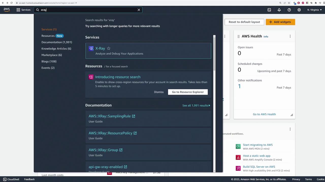
In this lesson, we explore how to leverage AWS X-Ray for analyzing application traces. The demonstration outlines working with the AWS X-Ray console to visualize, filter, and diagnose issues in your application's performance. An application has already been created, deployed on AWS, and instrumented using X-Ray libraries to capture and send trace data. This guide explains how to navigate the X-Ray console, interpret trace segments, and filter trace data for troubleshooting purposes.

Getting Started

Start by searching for "X-Ray" in the AWS Management Console, where you will discover that the X-Ray service is integrated within CloudWatch.

If you navigate to CloudWatch, you will notice a dedicated section for X-Ray. This section is organized into two subsections: Service Map and Traces.

Exploring the Service Map

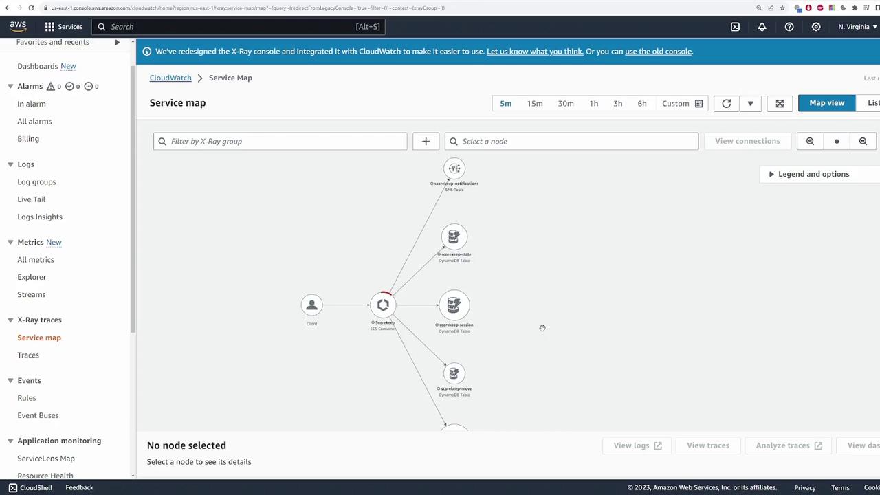
The Service Map provides a visual diagram detailing the interconnected components of your application. In the diagram below, the client (front-end user) sends a request to the scorekeep application running on an ECS container. This container then interacts with various components, such as:

• The scorekeep notification SNS topic
• Multiple DynamoDB tables for state, session, move, and game data

These interactions are clearly represented in the trace.

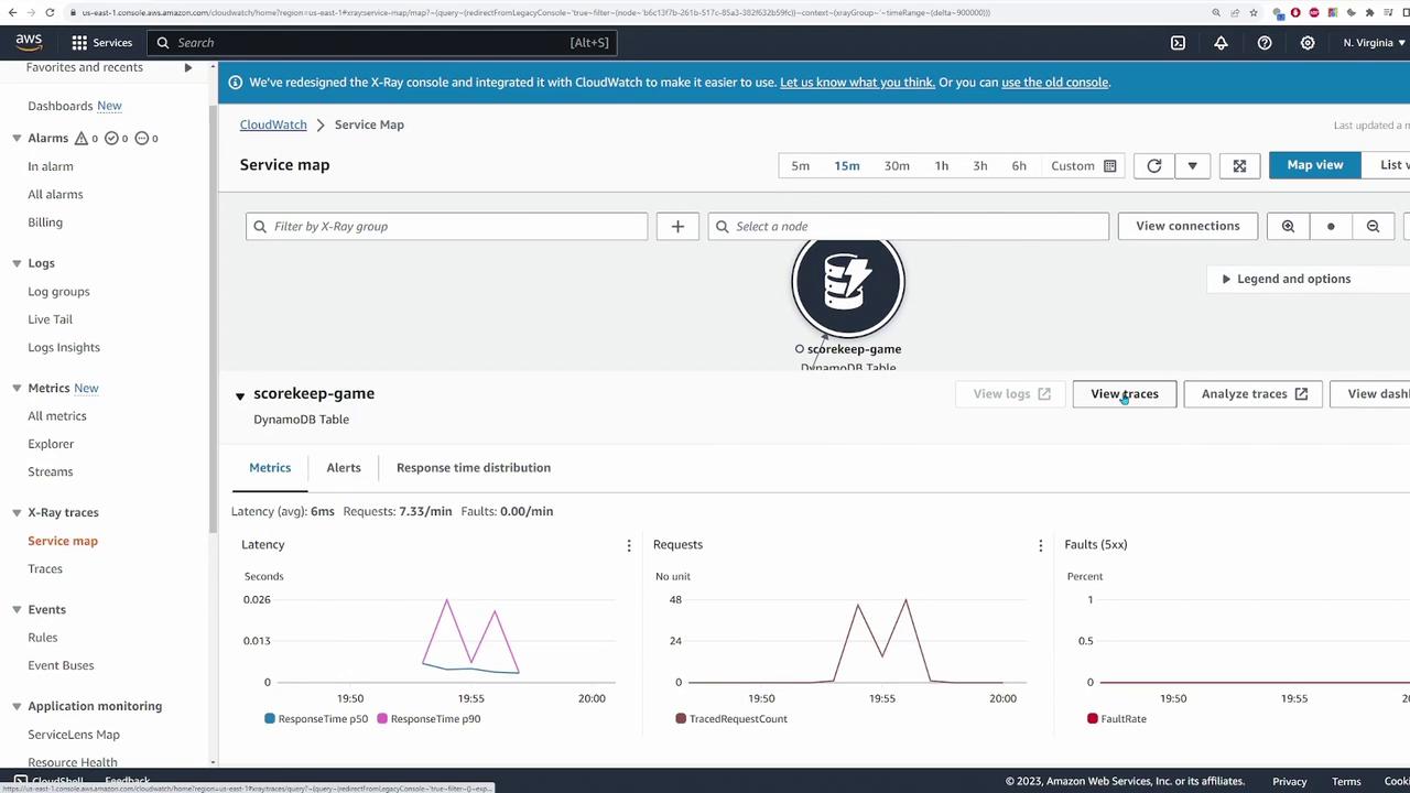
At the top of the interface, select a time frame (e.g., last 5 minutes or last 15 minutes). Clicking on a specific node will display all the traces involving that node. For instance, clicking a node reveals metrics like latency, request counts, total faults (including 500 status code failures), and response time distributions.

The dashboard below highlights how metrics and traces are presented. Traces with failures or errors are emphasized, enabling rapid identification of problematic segments.

Analyzing Individual Traces

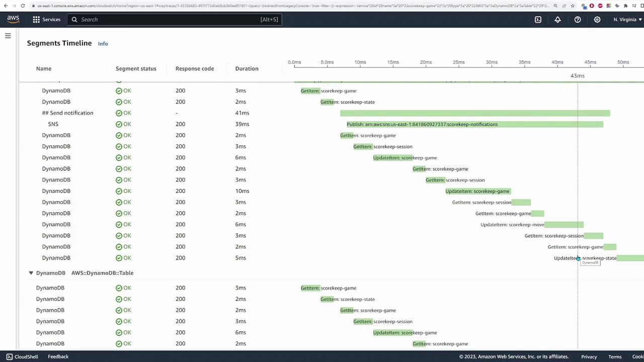
When you click on a trace, you will see the individual segments that form it. For example, a trace might begin with a request from your ECS container that interacts with the scorekeeping game table. In a simple trace, operations such as a "get item" on a DynamoDB table are segmented along with their durations.

Consider the following query that captures a segment related to the scorekeep game table:

service(id:{name:"scorekeep-game", type:"AWS::DynamoDB::Table"})

This query indicates that the application sends a get item request to the scorekeep game table, in addition to performing operations like retrieving an item from the scorekeep state table and sending an SNS notification. By examining the duration of each segment, you can pinpoint operations that may be increasing overall latency.

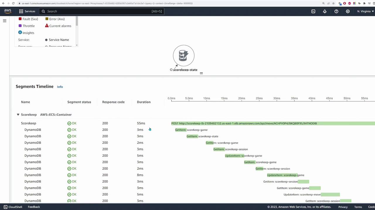
If a fault occurs (for example, a 500 error), the trace will highlight the location of the failure. The diagram below identifies a fault in the "Scorekeep" service, making it easier to isolate the problematic component.

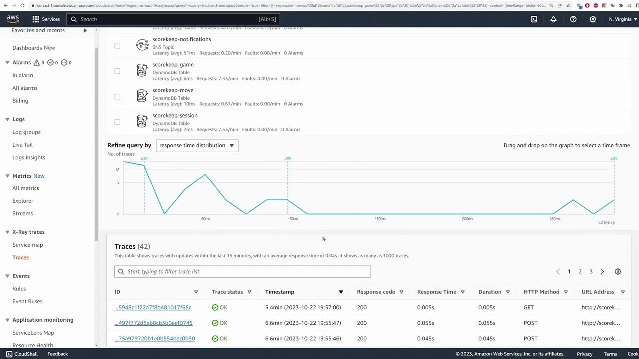
To view all traces within the selected time frame without filtering for a specific component, simply remove the current filter query and execute the query again. This will provide a comprehensive list of all captured traces. You can then click on each segment to view detailed information such as response codes and operation durations (e.g., 3 milliseconds, 2 milliseconds, etc.).

Moreover, refine your queries by selecting specific nodes. For example, adding a filter for traces that involve both the SNS topic and the scorekeep game table may yield a detailed list of 43 traces, complete with response time distributions and additional metrics.

Conclusion

This lesson demonstrates how AWS X-Ray serves as a powerful tool for tracing and monitoring your applications. By instrumenting your application with X-Ray and analyzing trace data in CloudWatch, you gain valuable insights into the journey of a request, allowing you to identify bottlenecks and enhance performance.

For more information on AWS X-Ray, consider exploring the following resources:

• AWS X-Ray Documentation
• CloudWatch Documentation

Thank you for reading this demonstration. We hope you found this step-by-step guide helpful, and we look forward to sharing more advanced lessons in the future.