Additional Training Methods

In this article, we explore advanced techniques to enhance and optimize model training in PyTorch. These additional methods—such as transfer learning, using PyTorch Hub for model sharing, and employing learning rate schedulers—help overcome common challenges like limited data, long training times, and unstable learning processes.

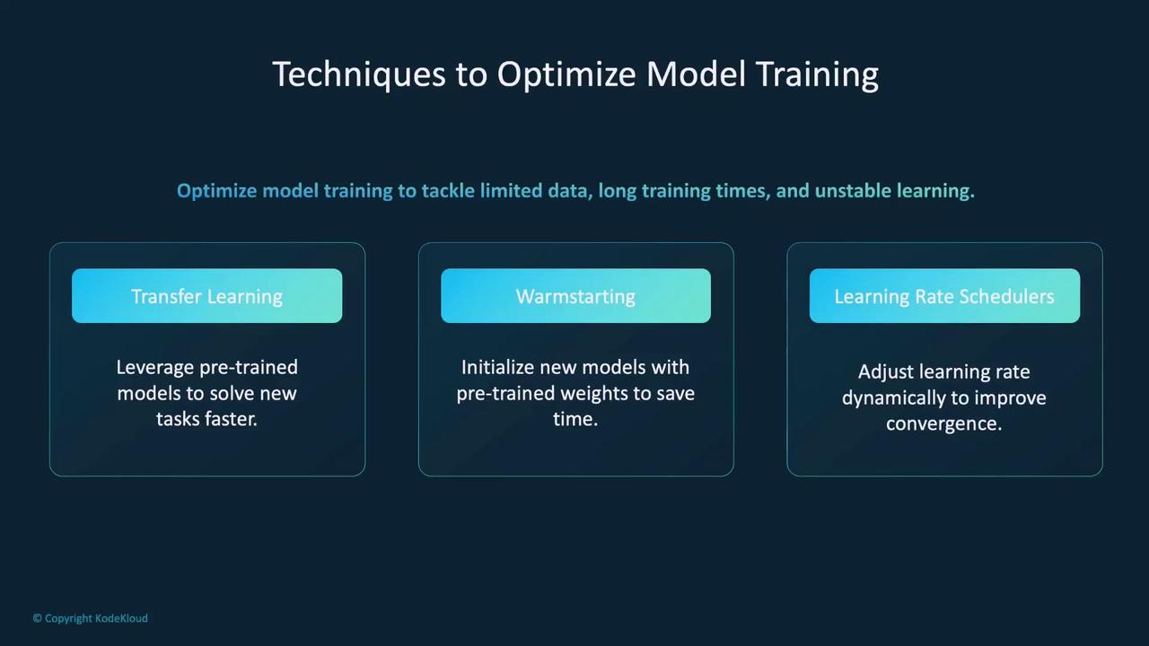
Let's dive in.

Additional training methods extend basic training approaches by integrating advanced strategies that save time and computational resources. Below are some key techniques:

• Transfer Learning: Leveraging pre-trained models for new or related tasks.
• Warm Starting: Initializing models with pre-trained weights to accelerate training.
• Learning Rate Schedulers: Dynamically adjusting the learning rate for better convergence.

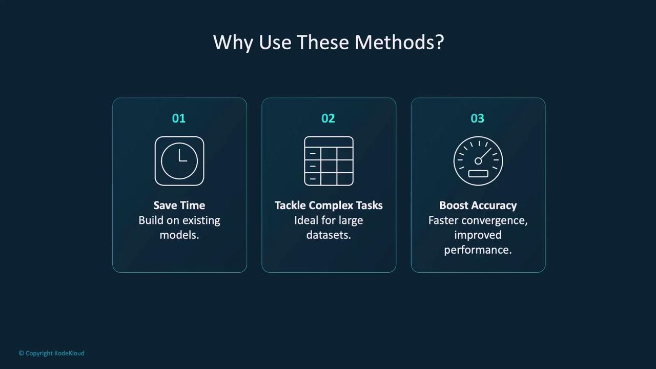
The primary advantage of these techniques is their ability to reduce training time and conserve resources by building on pre-existing models and recognized features. This is especially beneficial when working with large datasets or complex tasks.

Transfer Learning

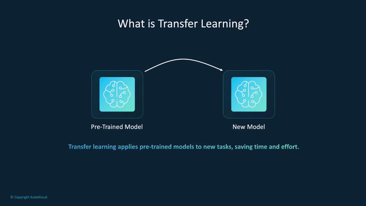
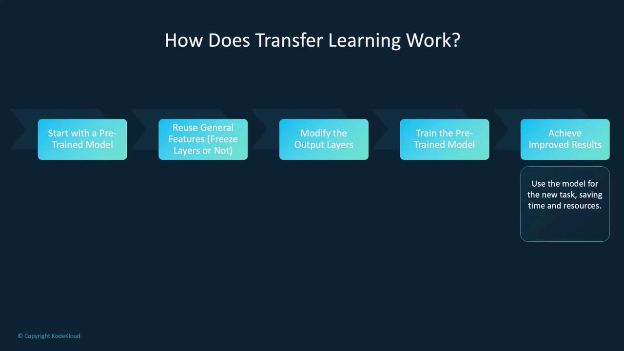
Transfer learning repurposes pre-trained models for new or similar tasks. By starting with a model trained on a large dataset (such as ImageNet), you can significantly reduce the training time for your own application.

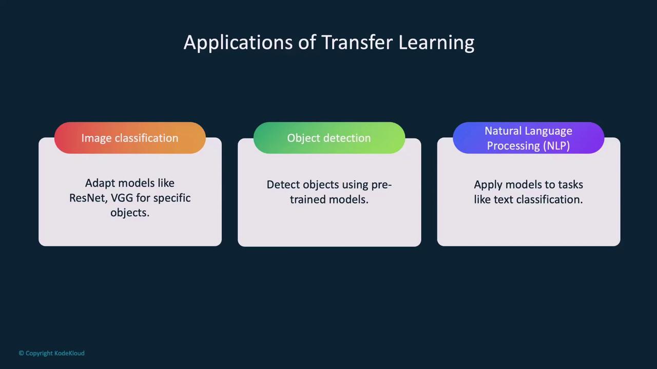
A pre-trained model has already learned foundational features—such as edges, textures, and more complex patterns—that can be reused for your specific task. This results in faster convergence during training, particularly when available data is limited. Transfer learning excels in domains such as image classification, object detection, and natural language processing.

How Transfer Learning Works

The initial layers of a pre-trained model capture generic features common to many tasks. Depending on your dataset size and the similarity between tasks, you can either freeze these layers or fine-tune the entire network.

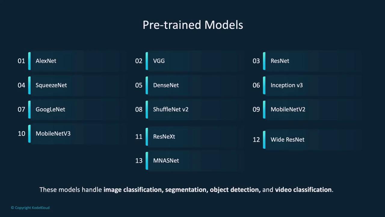
Since this article focuses on image classification, here are some popular pre-trained models available through TorchVision. These models support a range of tasks including image classification, segmentation, object detection, and video classification.

For instance, you can load these models directly using the following Python code:

import torchvision.models as models

# Load parameters from pre-trained models
resnet18 = models.resnet18(pretrained=True)
alexnet = models.alexnet(pretrained=True)
squeezenet = models.squeezenet1_0(pretrained=True)
vgg16 = models.vgg16(pretrained=True)
densenet = models.densenet161(pretrained=True)
inception = models.inception_v3(pretrained=True)
googlenet = models.googlenet(pretrained=True)
shufflenet = models.shufflenet_v2_x1_0(pretrained=True)
mobilenet_v2 = models.mobilenet_v2(pretrained=True)
mobilenet_v3_large = models.mobilenet_v3_large(pretrained=True)
mobilenet_v3_small = models.mobilenet_v3_small(pretrained=True)
resnext50_32x4d = models.resnext50_32x4d(pretrained=True)
wide_resnet50_2 = models.wide_resnet50_2(pretrained=True)
mnasnet = models.mnasnet1_0(pretrained=True)

Modifying a Pre-Trained Model

The example below demonstrates how to adapt a pre-trained ResNet-18 model for a new task involving 10 output classes:

import torch.nn as nn
import torchvision.models as models

# Load the pre-trained ResNet-18 model
model = models.resnet18(pretrained=True)

# Get the number of features in the last fully connected layer
num_ftrs = model.fc.in_features

# Replace the fully connected layer for a new task with 10 classes
model.fc = nn.Linear(num_ftrs, 10)

Here, the final fully connected layer is replaced with a new one that outputs predictions for 10 classes. The number of input features is obtained from the original model's configuration.

PyTorch Hub

PyTorch Hub is a community-driven platform that provides access to a wide range of pre-trained models. It simplifies the process of exploring, downloading, and sharing models contributed by researchers around the world.

To browse available models, use the torch.hub.list function by specifying the GitHub repository. For example, to list vision models from the PyTorch/vision repository, execute:

# List vision models available from the PyTorch/vision repository
torch.hub.list('pytorch/vision')
Downloading: "https://github.com/pytorch/vision/zipball/main" to .cache/torch/hub/main.zip
['alexnet', 'convnext_base', 'convnext_large', 'convnext_small', 'convnext_tiny',
 'deeplabv3_mobilenet_v3_large', 'deeplabv3_resnet50',
 'densenet121', 'densenet161', 'densenet169', 'densenet201', 'efficientnet_b0',
 'efficientnet_b1', 'efficientnet_b2', 'efficientnet_b3', 'efficientnet_b4',
 'efficientnet_b5', 'efficientnet_b6', 'efficientnet_b7', 'efficientnet_v2_l',
 'efficientnet_v2_m', 'efficientnet_v2_s', 'fcn_resnet101', 'fcn_resnet50',
 'get_model_weights', 'get_weight', 'googlenet', 'inception_v3',
 'lrappt_mobilenet_v3_large', 'maxvit_t', 'mc3_18', 'mnasnet0_5', 'mnasnet0_75',
 'mnasnet1_0', 'mnasnet1_3', 'mobilenet_v2', 'mobilenet_v3_large',
 'mobilenet_v3_small', 'mvit_v1_b', 'mvit_v2_s', 'r2plus1d_18', 'r3d_18',
 'raft_large', 'raft_small', 'regnet_x_16gf', 'regnet_x_1_6gf', 'regnet_x_32gf']

After identifying the desired model, load it using the torch.hub.load function. For example, to load the pre-trained VGG-16 model:

import torch

# Load pre-trained VGG-16 model
model = torch.hub.load('pytorch/vision', 'vgg16')
print(model)

PyTorch Hub also enables model deployment by facilitating model sharing. To share your model, create a file named hubconf.py in your repository. This file defines the entry point for your model. The following example illustrates how to set up a hubconf.py for a ResNet-18 model:

dependencies = ['torch']
from torchvision.models.resnet import resnet18 as resnet

def model(pretrained=False, **kwargs):
    """ResNet-18 model
    pretrained (bool): Load pretrained weights if True.
    """
    # Initialize the model with optional pretrained weights
    model = resnet(pretrained=pretrained, **kwargs)
    if pretrained:
        checkpoint = 'https://model-url.pth'
        state_dict = torch.hub.load_state_dict_from_url(checkpoint, progress=False)
        model.load_state_dict(state_dict)
    return model

Users can then load the shared model using:

# Load the model from a GitHub repository
model = torch.hub.load('username/repo_name', 'model', pretrained=True)

Learning Rate Schedulers

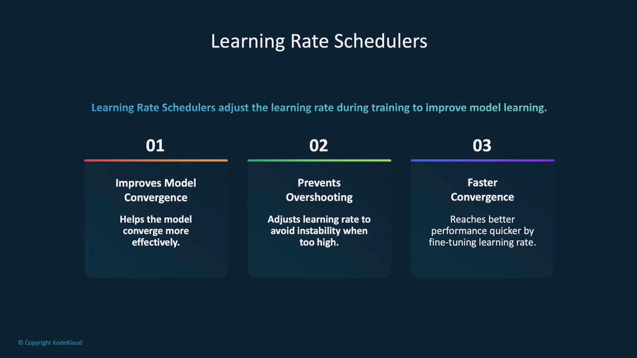
Learning rate schedulers play a crucial role in training by adjusting the learning rate throughout the training process. This dynamic adjustment ensures that the model takes larger steps in the early stages and fine-tuned adjustments later, preventing issues like overshooting optimal parameters.

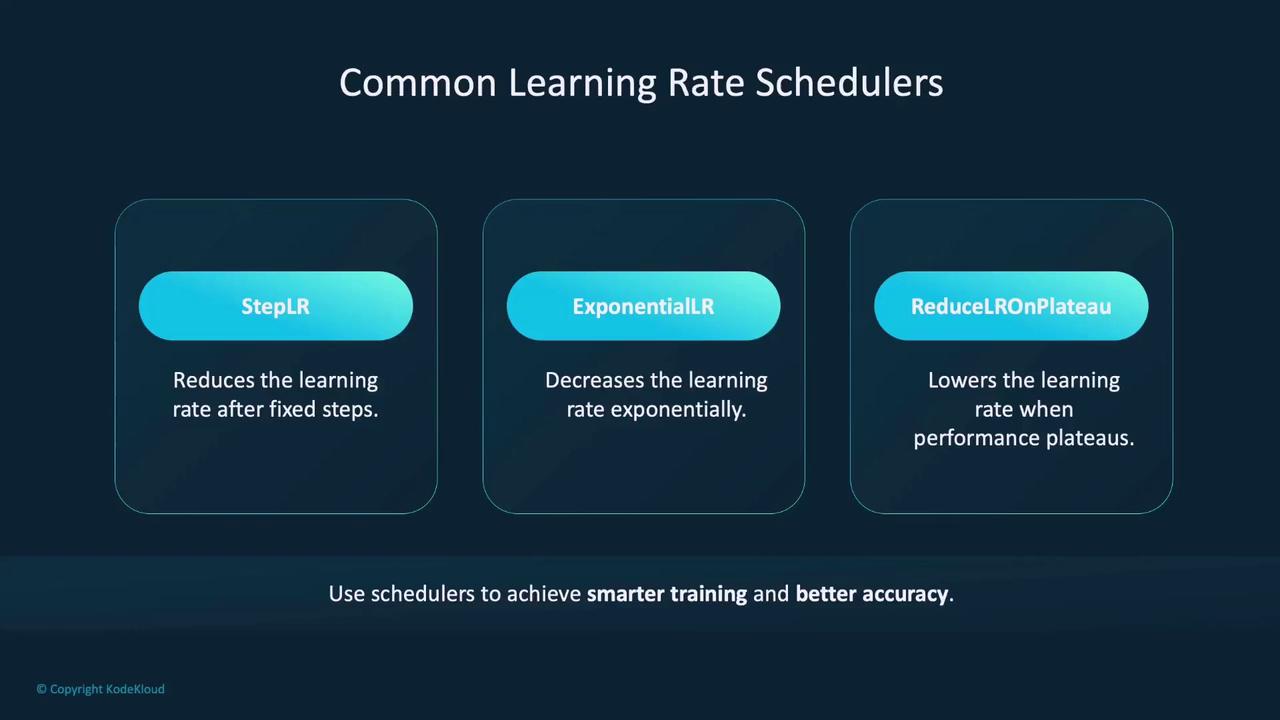
PyTorch provides several built-in learning rate schedulers:

• StepLR: Decreases the learning rate by a fixed factor (gamma) after a set number of epochs.
• ExponentialLR: Applies an exponential decay to the learning rate.
• ReduceLROnPlateau: Lowers the learning rate when performance metrics stagnate.

To integrate a learning rate scheduler into your training loop, first define an optimizer, then configure the scheduler, and finally update it at the end of each epoch. For instance, to use a StepLR scheduler with an SGD optimizer:

import torch.optim as optim

# Define the optimizer with an initial learning rate
optimizer = optim.SGD(model.parameters(), lr=0.01)

# Configure the StepLR scheduler to decay the learning rate every 10 epochs by a factor of 0.1
scheduler = optim.lr_scheduler.StepLR(optimizer, step_size=10, gamma=0.1)

# Training loop
for epoch in range(50):
    # Insert your training logic here
    # ...

    # Update the learning rate at the end of the epoch
    scheduler.step()

Summary

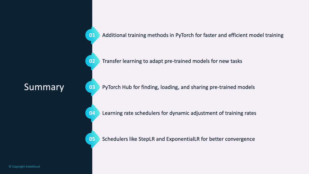
In summary, this article has covered several advanced training methods in PyTorch:

• Transfer Learning: Utilize pre-trained models to achieve faster convergence and reduce training time.
• PyTorch Hub: Access and share a wide range of pre-trained models through a community-driven platform.
• Learning Rate Schedulers: Dynamically adjust learning rates during training to avoid overshooting and ensure efficient convergence.

These techniques are invaluable for building complex models with enhanced accuracy and efficiency. Next, let's move on to the demonstration section to see these methods in action.