PyTorch

Building and Training Models

Model Evaluation

In this lesson, we trained three distinct models: a custom model from scratch and two models leveraging transfer learning. Now, we need to select the best candidate for deployment in production. Before making that decision, a thorough model evaluation must be performed.

The image is a flowchart comparing three models: "Custom Model from Scratch," "Transfer Learning Model 1," and "Transfer Learning Model 2," with the latter being selected for model evaluation and deployment.

Model evaluation is the process of assessing a machine learning model's performance on unseen data. It verifies whether the model has effectively captured the underlying patterns in the training data and can generalize to new examples. Think of it as administering a test to the model using questions it hasn't seen before.

To perform the evaluation, we use a separate dataset—commonly known as the test dataset—which is not used during the training phase. By comparing the model's predictions with the true labels, we can determine its effectiveness.

The image is a slide titled "Introduction to Model Evaluation," highlighting two key points: assessing model performance on unseen data and ensuring effective pattern learning and generalization.

The image is a flowchart titled "Introduction to Model Evaluation," showing the process from "Test Data" to "ML Model" to "Predictions."

This evaluation process enables us to compute metrics such as accuracy—which reflects how many predictions are correct—as well as precision and recall, which provide more detailed insights especially when dealing with imbalanced datasets.

The image is an introduction to model evaluation, showing a flow between predictions and correct answers, and explaining that accuracy shows correct predictions while precision and recall assess detection of specific events.

Evaluating a model is crucial because a model that performs exceptionally well on training data might still fail in real-world scenarios due to overfitting. Overfitting happens when the model memorizes the training data rather than learning generalizable patterns. By rigorously testing on unseen data, we can detect such issues and choose the model that best meets our operational requirements.

The image outlines the importance of model evaluation, highlighting three points: ensuring models generalize beyond training data, detecting overfitting and genuine learning, and comparing models to find the best fit.

It also helps pinpoint weaknesses, such as difficulty handling specific input types, thereby allowing us to make necessary improvements before deployment.

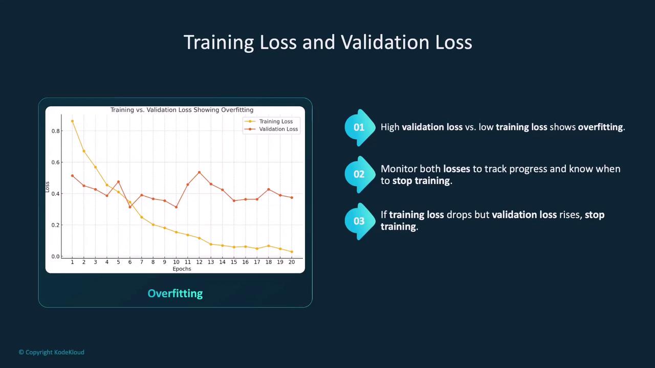
Training vs. Validation Loss

During model training, we compute two key loss metrics: training loss and validation loss. These metrics provide insights into how well the model learns from the provided data.

  • Training Loss: This metric measures error on the training dataset, which the model uses to iterate and optimize its parameters through methods like gradient descent. A low training loss indicates that the model is learning from the training data, but it doesn't guarantee good generalization.

  • Validation Loss: This loss is computed on an unseen validation dataset after each training epoch (without updating the model parameters). A large discrepancy between training and validation loss is a strong indicator of overfitting.

Monitoring these metrics together helps in deciding when to stop the training process. If training loss decreases continually while validation loss increases, it signifies that the model is overfitting.

The image shows a graph comparing training and validation loss over epochs, illustrating overfitting, along with three key points about monitoring these losses during model training.

A balanced training approach will yield similar training and validation loss values over time.

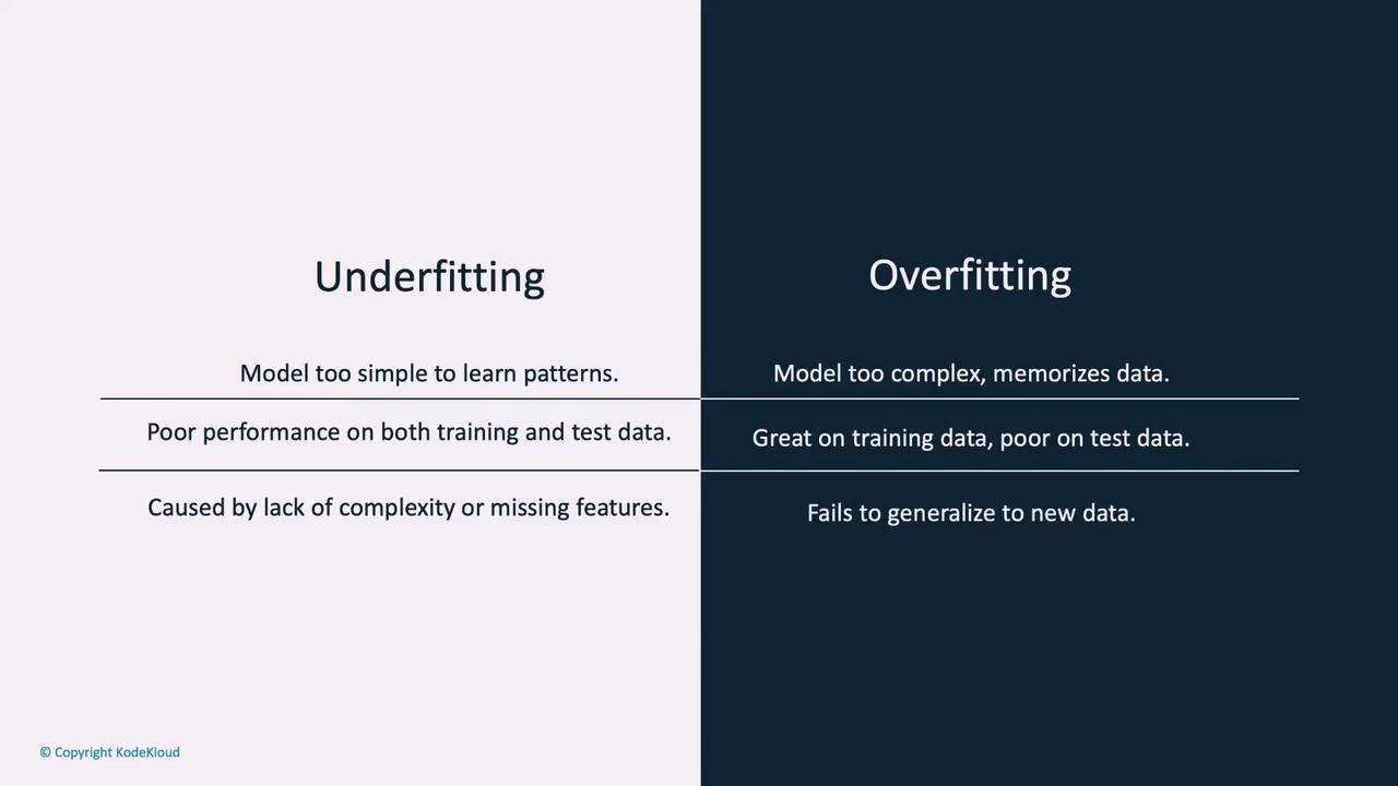
Overfitting vs. Underfitting

Two common challenges during model training are overfitting and underfitting:

  • Underfitting: Occurs when the model is too simple to capture the underlying trends in the data, resulting in poor performance on both training and test datasets.

  • Overfitting: Happens when a model is overly complex and starts to memorize the training data instead of learning generalizable patterns. Even though it might perform excellently on the training set, its performance on new, unseen data deteriorates.
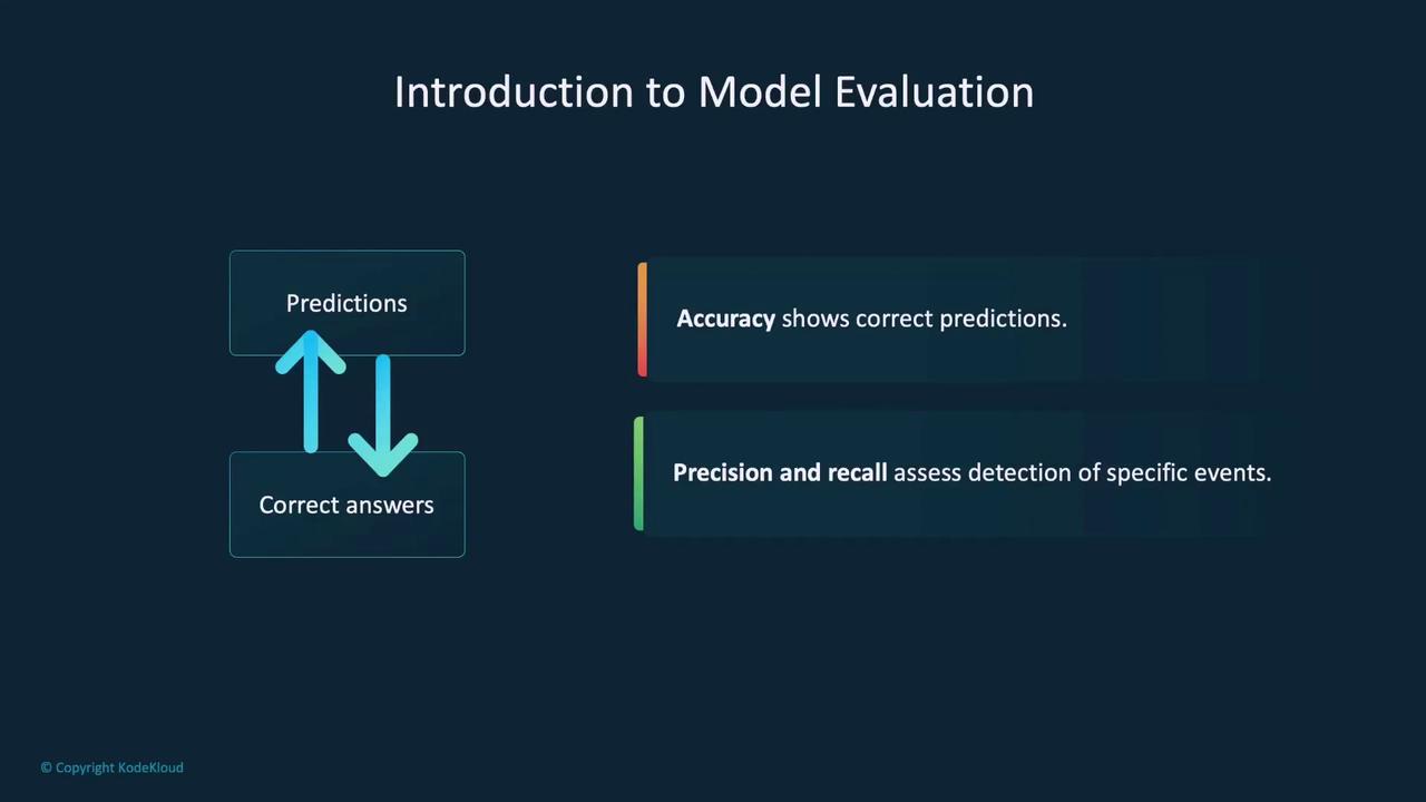
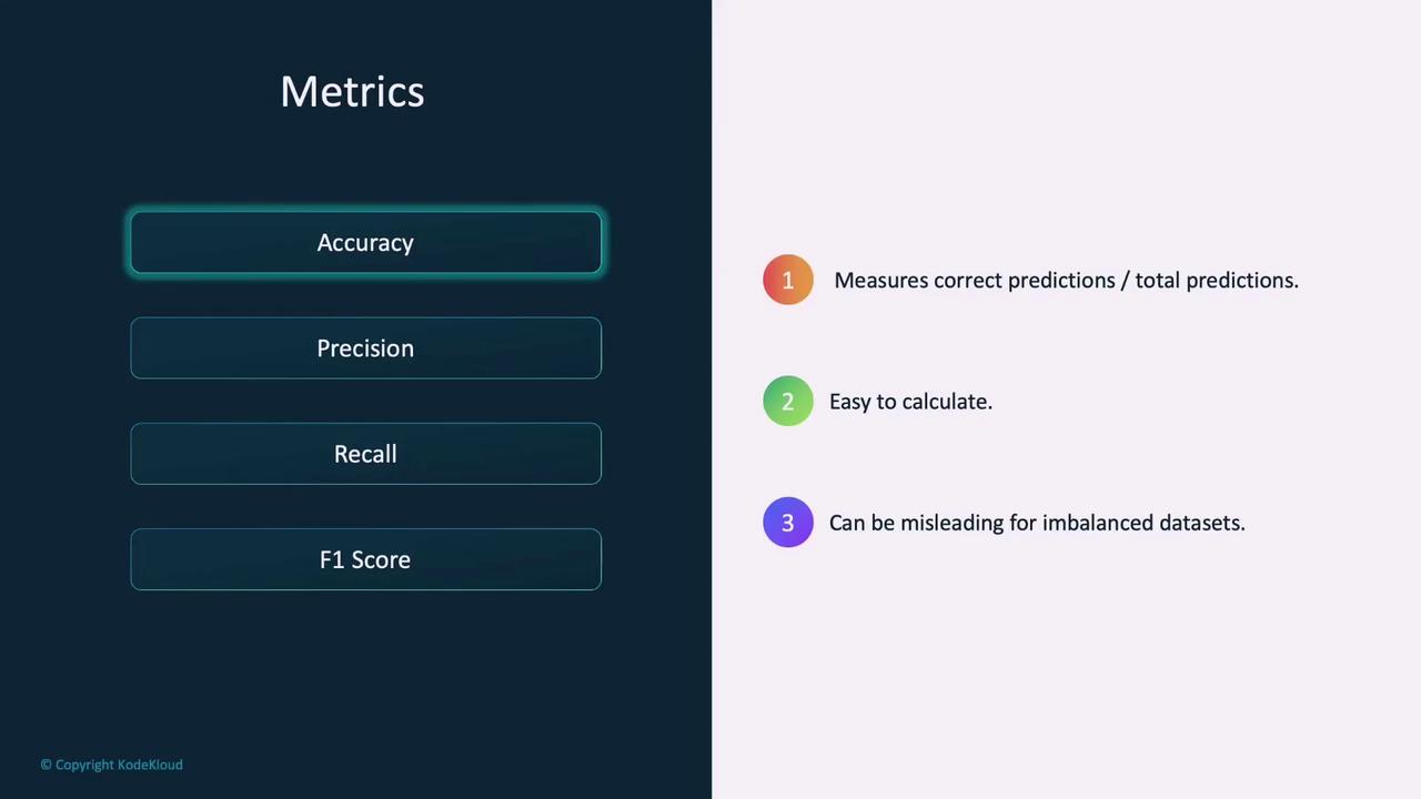
The image compares underfitting and overfitting in machine learning models, highlighting their characteristics and effects on data performance.

The goal is to strike a balance where the model can generalize well without falling into the traps of underfitting or overfitting.

Evaluation Metrics

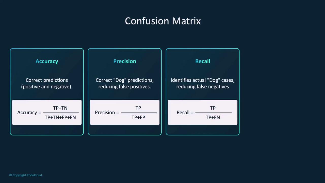
Model evaluation employs several metrics to quantify performance:

  • Accuracy: Represents the ratio of correctly predicted instances to the total predictions. While accuracy is easy to compute, it can be misleading for imbalanced datasets.

    The image is a slide titled "Metrics" listing four metrics: Accuracy, Precision, Recall, and F1 Score, with a focus on Accuracy, explaining it as the ratio of correct predictions to total predictions, noting it's easy to calculate but can be misleading for imbalanced datasets.

  • Precision: Indicates the ratio of true positive predictions to all positive predictions made by the model. This metric is vital in scenarios where false positives carry a high cost, such as spam detection or medical diagnosis.

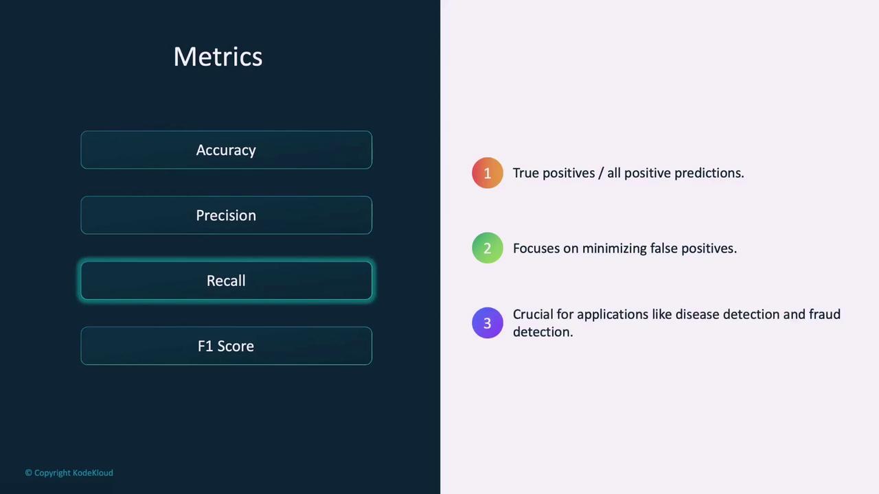
  • Recall: Denotes the ratio of true positive predictions to all actual positive cases, focusing on the model's ability to identify all positive instances. It is especially important in fields like disease detection and fraud monitoring.

    The image shows a list of metrics including Accuracy, Precision, Recall, and F1 Score, with a focus on Recall, explaining its importance in minimizing false positives and its application in fields like disease and fraud detection.

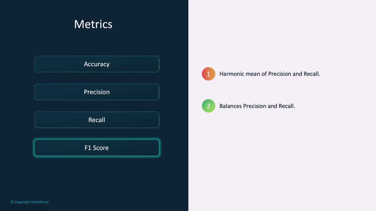
  • F1 Score: This is the harmonic mean of precision and recall. It provides a single metric that balances both false positives and false negatives, making it useful when you need a balance between precision and recall.

    The image shows a list of metrics including Accuracy, Precision, Recall, and F1 Score, with a focus on F1 Score, described as the harmonic mean of Precision and Recall, balancing both.

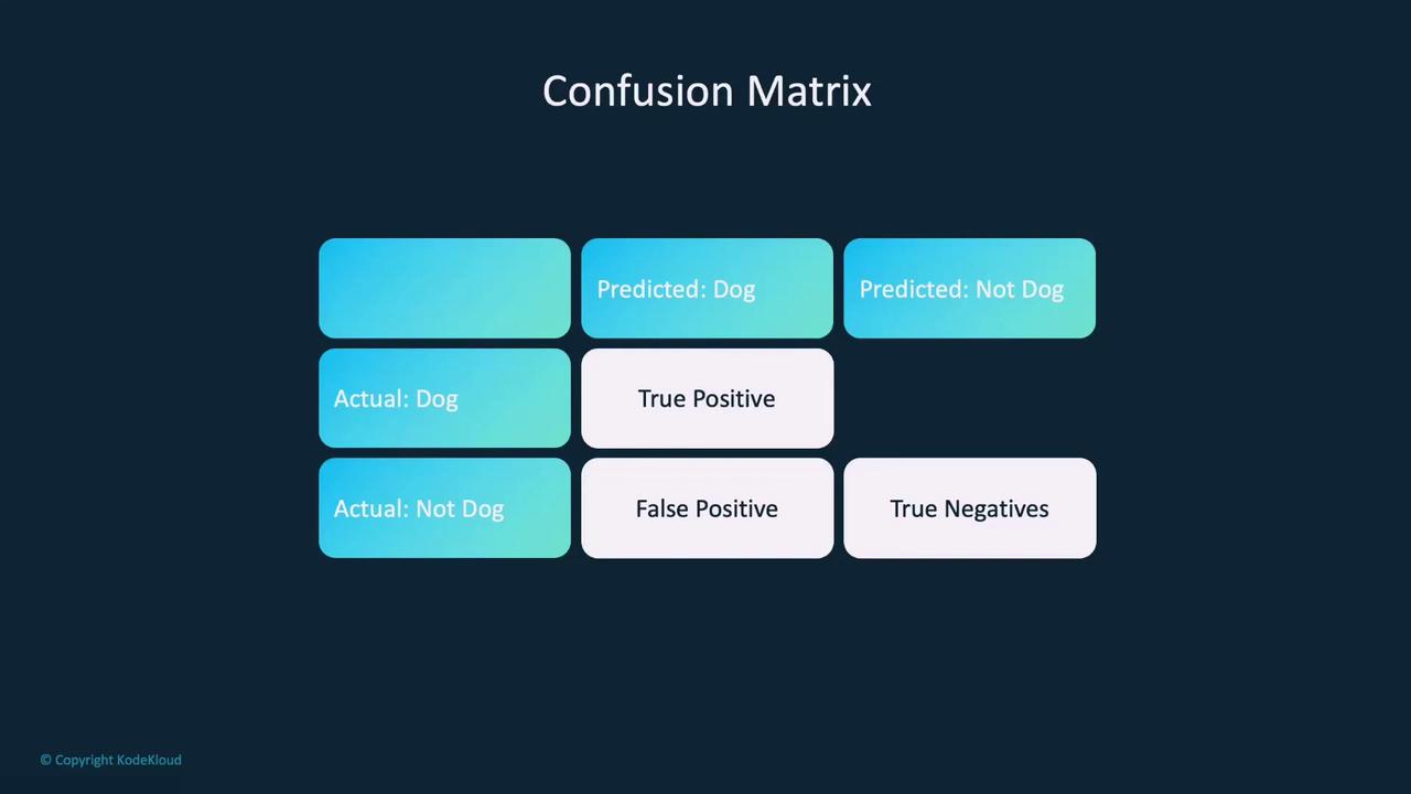
The Confusion Matrix

A confusion matrix is an essential tool for evaluating classification models. It offers a detailed breakdown by comparing actual labels with the model’s predictions and categorizing them as follows:

  • True Positives: Both predicted and actual labels are positive (e.g., both are "dog").
  • True Negatives: Both predicted and actual labels are negative.
  • False Positives: The model predicts positive while the actual label is negative.
  • False Negatives: The model predicts negative while the actual label is positive.

The image is a confusion matrix illustrating predictions of "Dog" and "Not Dog" with categories for true positives, false positives, and true negatives.

This matrix is the foundation for computing metrics like accuracy, precision, and recall.

The image is a diagram explaining a confusion matrix, detailing the concepts of accuracy, precision, and recall with their respective formulas.

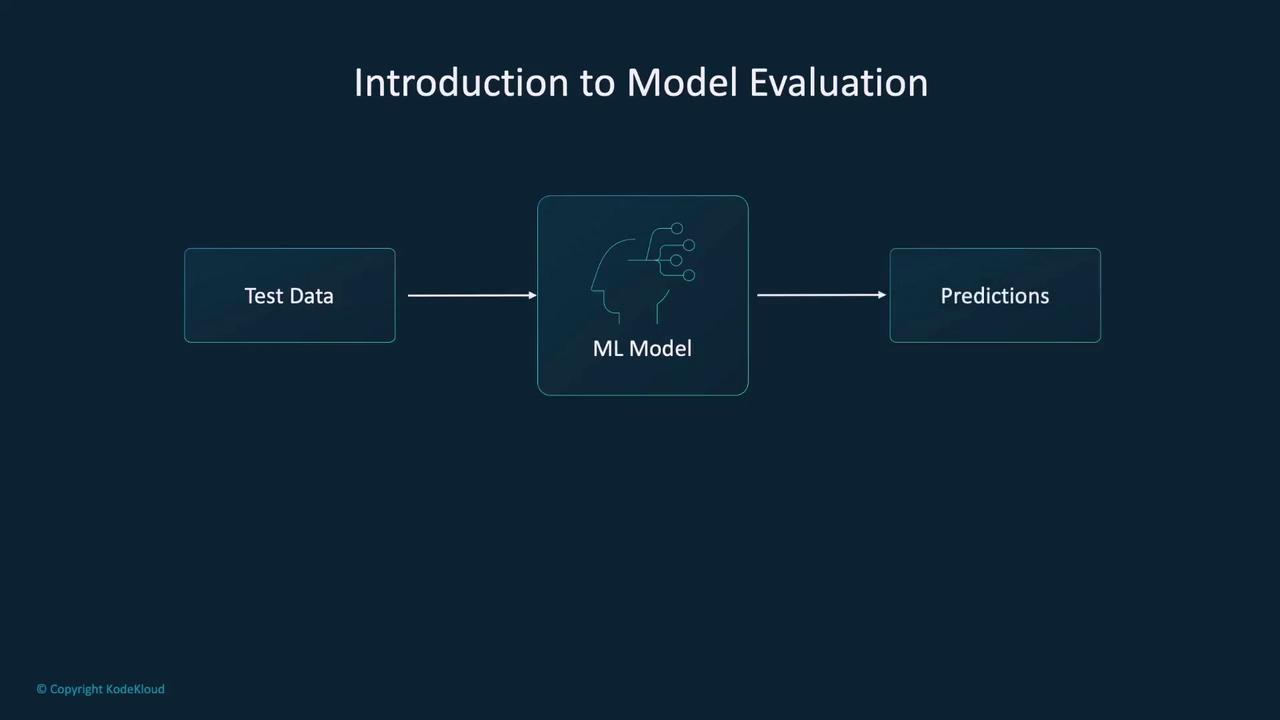
Model Evaluation in Practice

Evaluating a model often mirrors the approach used during training, but with key distinctions. In evaluation, we use a test loop where gradient computation is disabled using PyTorch’s no_grad function. This approach reduces memory usage and enhances computational speed.

Below is an example showcasing both a training loop (for context) and a test loop used for evaluation:

# Training Loop
for epoch in range(N_EPOCHS):
    running_loss = 0.0
    for i, data in enumerate(train_loader, 0):
        inputs, labels = data
        optimizer.zero_grad()
        outputs = model(inputs)
        loss = criterion(outputs, labels)
        loss.backward()
        optimizer.step()
        running_loss += loss.item()
    print(f"Epoch: {epoch} Loss: {running_loss / len(train_loader)}")

# Test Loop
model.eval()  # Set the model to evaluation mode
with torch.no_grad():  # Disable gradient computation
    for i, data in enumerate(test_loader, 0):
        inputs, labels = data
        outputs = model(inputs)
        _, preds = torch.max(outputs.data, 1)

# Metric calculation
print("metric calculation:")

In the test loop, the separate test_loader dataset is used to evaluate the model on unseen data. The use of torch.no_grad() is crucial as it temporarily disables gradient tracking during inference, significantly reducing memory consumption.
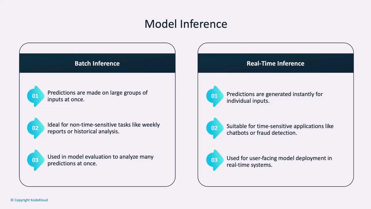
Inference Paradigms

There are two primary paradigms for model inference:

  • Batch Inference: This approach processes predictions on a group of inputs at once, making it ideal for non-time-sensitive tasks like generating weekly reports or analyzing historical data. It allows for efficient processing of large datasets.

  • Real-Time Inference: In this scenario, predictions are generated instantly as individual inputs arrive. This method is critical for time-sensitive applications such as chatbots, fraud detection systems, or self-driving cars.

The image compares batch inference and real-time inference, highlighting their uses and ideal applications. Batch inference is suited for non-time-sensitive tasks, while real-time inference is for time-sensitive applications.

Integrating TorchMetrics for Evaluation

For more efficient metric computation in our test loop, we can integrate the TorchMetrics library. TorchMetrics simplifies tracking of key performance metrics in PyTorch. It provides pre-built functions for metrics such as accuracy, precision, recall, and F1 score, and is compatible with both CPU and GPU. You can also define custom metrics if needed.

The image is an informational graphic about "Torchmetrics," a Python library for calculating and tracking machine learning metrics, highlighting features like prebuilt metrics, PyTorch integration, and CPU/GPU support.

Below is an example of how to use TorchMetrics within a test loop:

import torchmetrics

# Initialize the accuracy metric for multiclass classification
accuracy_metric = torchmetrics.Accuracy(task="multiclass", num_classes=N)

# Test Loop
model.eval()  # Set model to evaluation mode
with torch.no_grad():  # Disable gradient computation
    for i, data in enumerate(test_loader, 0):
        inputs, labels = data
        outputs = model(inputs)
        _, preds = torch.max(outputs.data, 1)
        # Update the accuracy metric with predictions and true labels
        accuracy_metric.update(preds, labels)

# Compute and display the overall accuracy
accuracy = accuracy_metric.compute()
print(f"Accuracy: {accuracy!r}")

In this workflow, the accuracy metric keeps track of statistics over each batch, and after the evaluation loop completes, the overall accuracy is computed and displayed.

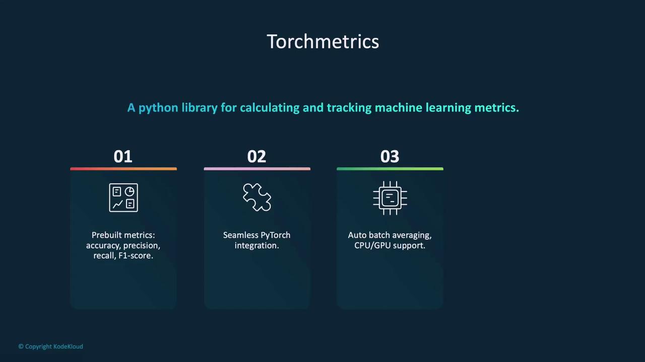
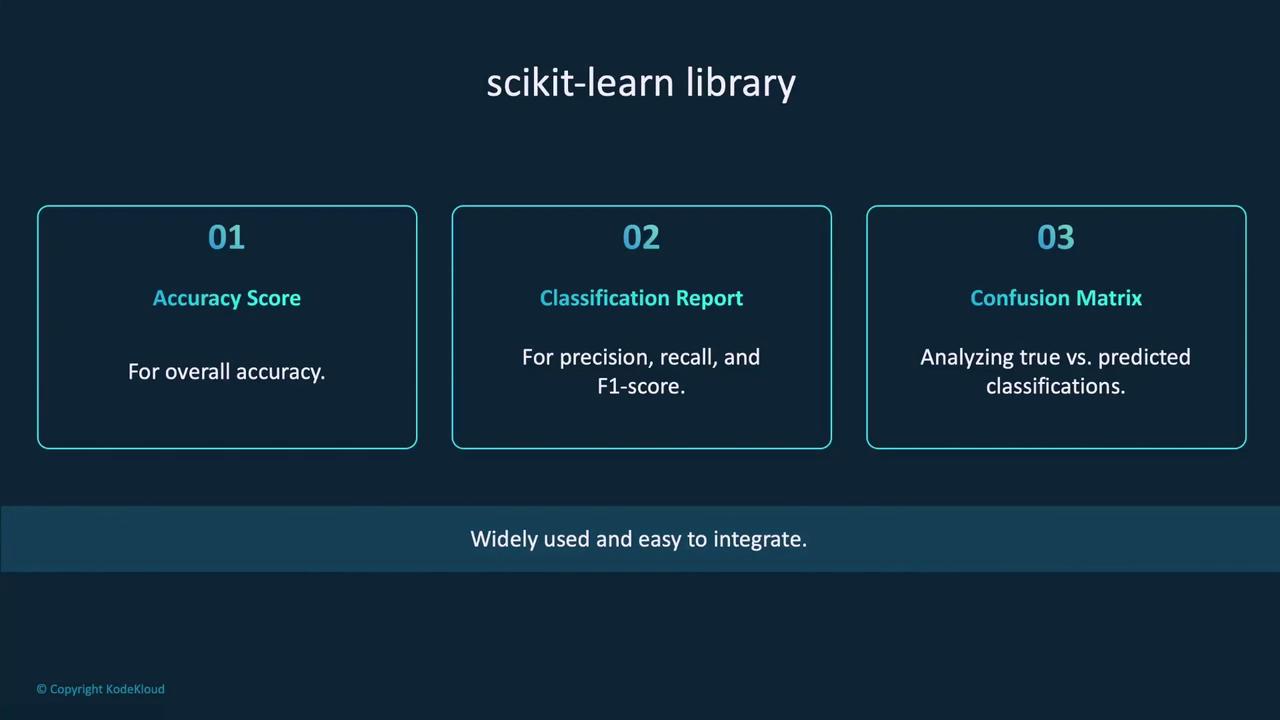
Alternative Evaluation Methods

In addition to TorchMetrics, other evaluation libraries such as Scikit-learn offer robust solutions and additional metrics:

  • Accuracy Score: For overall prediction accuracy.
  • Classification Report: Provides a detailed report including precision, recall, and F1 score.
  • Confusion Matrix: Offers a granular breakdown of true vs. predicted labels.
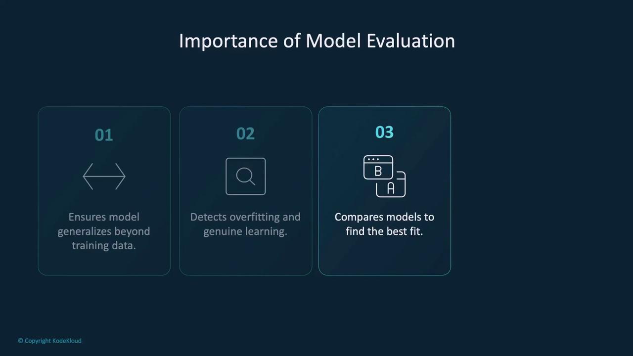
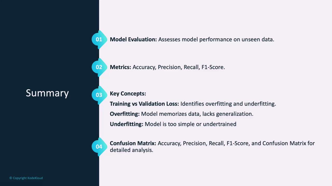
The image is an overview of the scikit-learn library, highlighting three features: Accuracy Score for overall accuracy, Classification Report for precision, recall, and F1-score, and Confusion Matrix for analyzing true vs. predicted classifications. It notes that the library is widely used and easy to integrate.

These alternative tools allow for flexible and comprehensive model evaluation tailored to specific needs.

Summary

In summary, model evaluation is critical for ensuring that a machine learning model generalizes well to unseen data. Key takeaways include:

  • Monitoring both training and validation losses to detect overfitting or underfitting.
  • Utilizing diverse evaluation metrics such as accuracy, precision, recall, and F1 score.
  • Leveraging tools like the confusion matrix for detailed analysis of the model's performance.
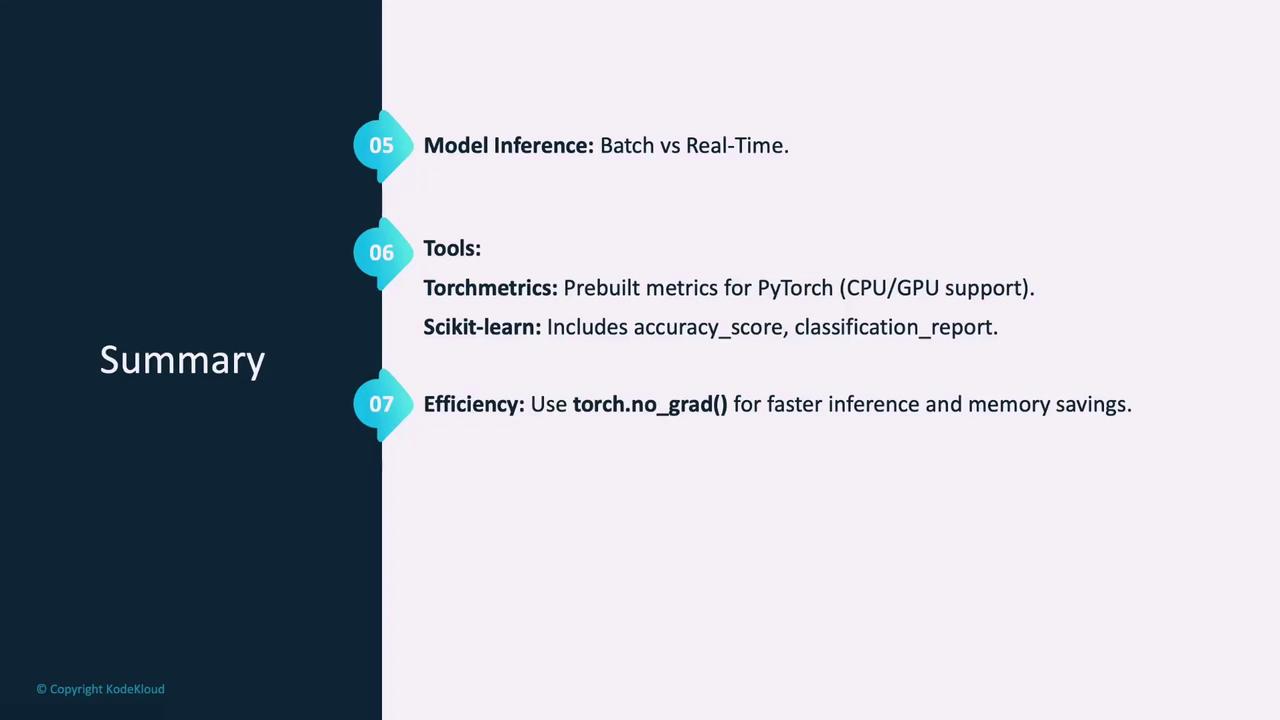
  • Integrating libraries such as TorchMetrics or Scikit-learn to streamline the evaluation process.
  • Understanding the distinction between batch and real-time inference based on application requirements.
  • Using PyTorch’s no_grad() function during evaluation to optimize memory usage and speed up inference.

The image is a summary slide outlining key concepts in model evaluation, including metrics like accuracy and precision, and concepts like overfitting and underfitting. It also mentions the use of a confusion matrix for detailed analysis.

The image is a summary slide discussing model inference, tools like Torchmetrics and Scikit-learn, and efficiency tips for PyTorch.

Note

For optimal model performance, always validate using multiple metrics and choose the evaluation strategy that aligns with your application's requirements.

This concludes our discussion on model evaluation. In the next demo, we will walk through the complete process—from running the test loop to computing the final metrics—to further solidify these concepts in practice.

Watch Video

Watch video content

Previous
Demo Additional Training Methods