- Core Concepts
- How Reinforcement Learning Works
- Markov Decision Processes (MDPs)
- Value-Based Methods
- Policy-Based & Actor-Critic Methods
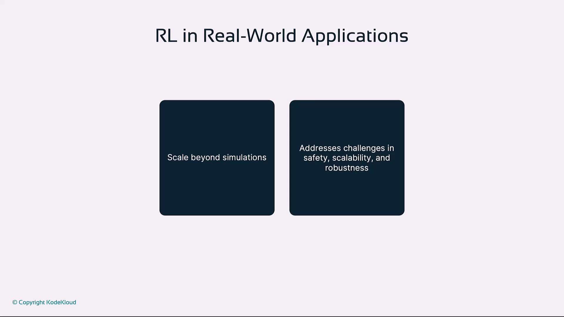
- Applications
- Challenges
- Future Directions
1. Core Concepts
An RL agent interacts with an environment in discrete time steps:| Term | Description |
|---|---|
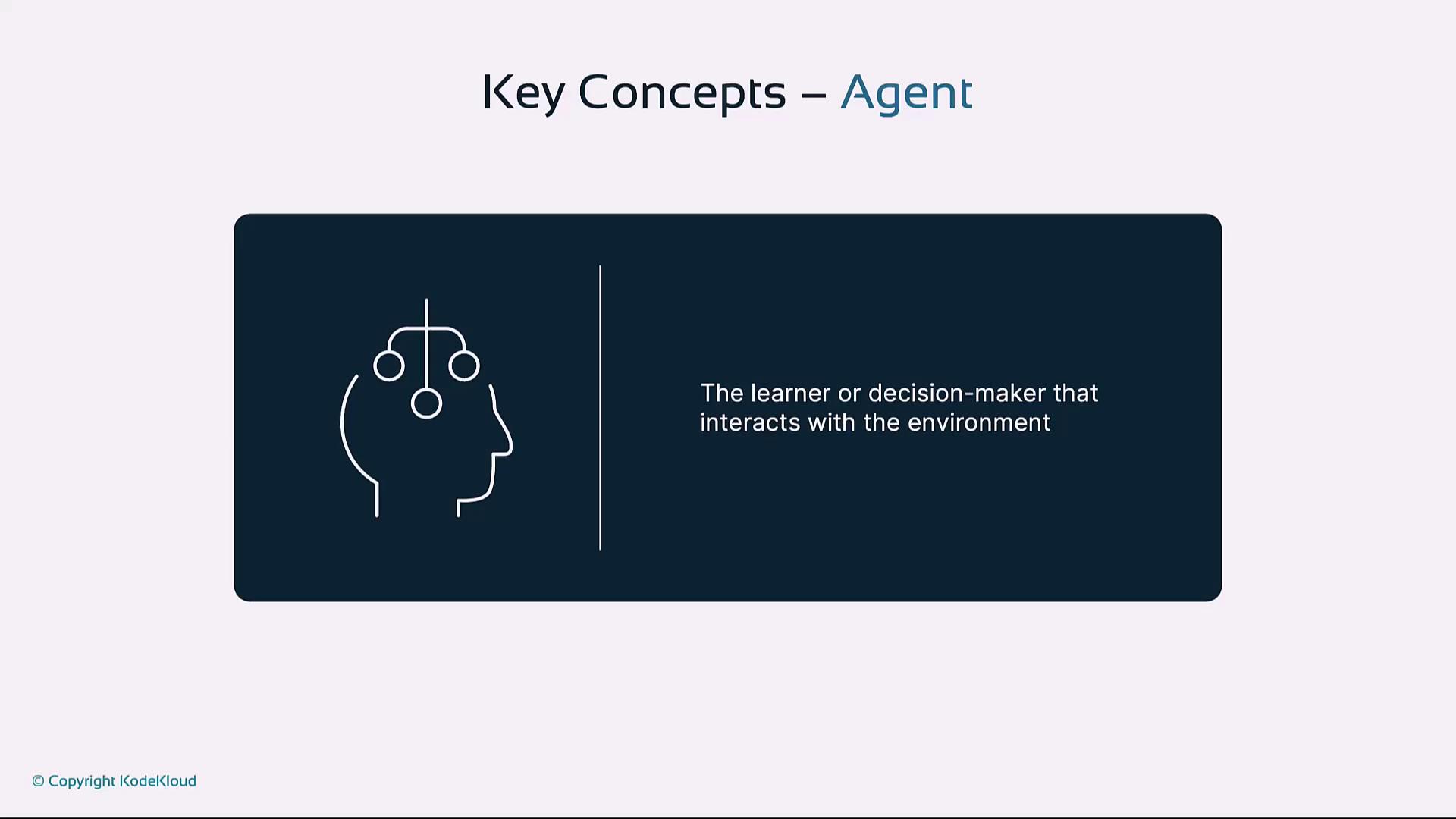
| Agent | The learner or decision-maker that selects actions |
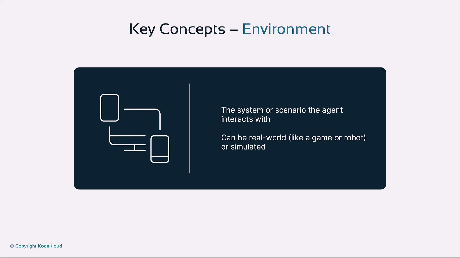
| Environment | The system or scenario (real or simulated) with which the agent interacts |
| State (S) | The current configuration of the environment observed by the agent |
| Action (A) | A decision or move the agent makes in a given state |
| Reward (R) | Immediate feedback indicating benefit or cost of an action |
| Policy (π) | Strategy mapping states to action probabilities |
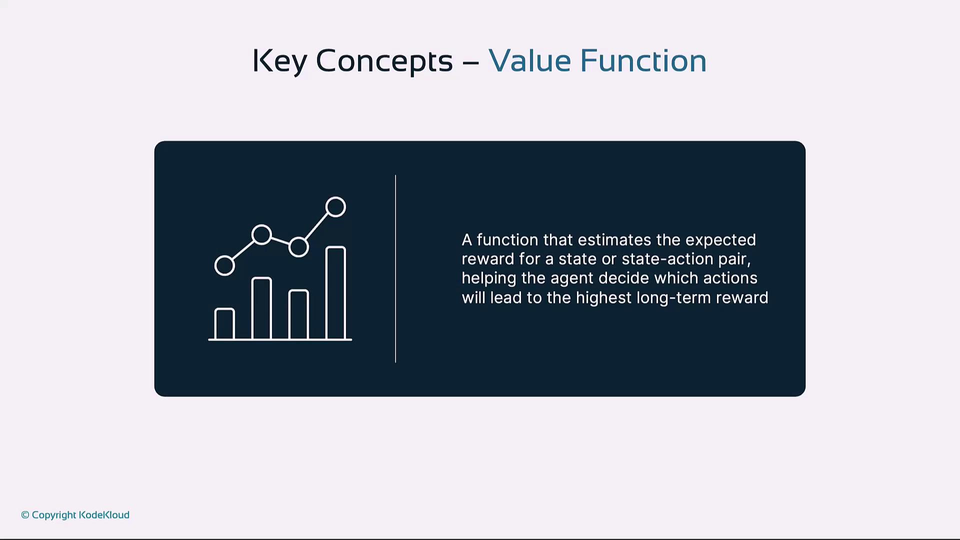
| Value Function | Estimates expected cumulative reward of states (or state–action pairs) |
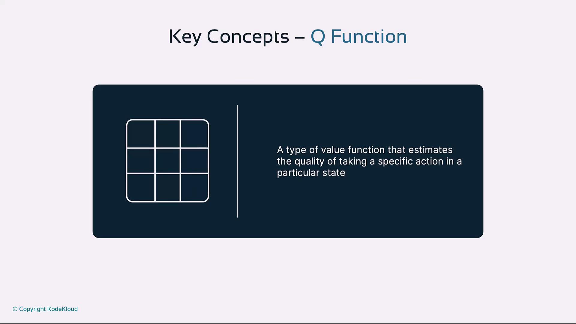
| Q-Function | A value function Q(s, a) estimating expected reward for action a in state s |
Agent
Environment
State
Reward
Value Function
Q-Function
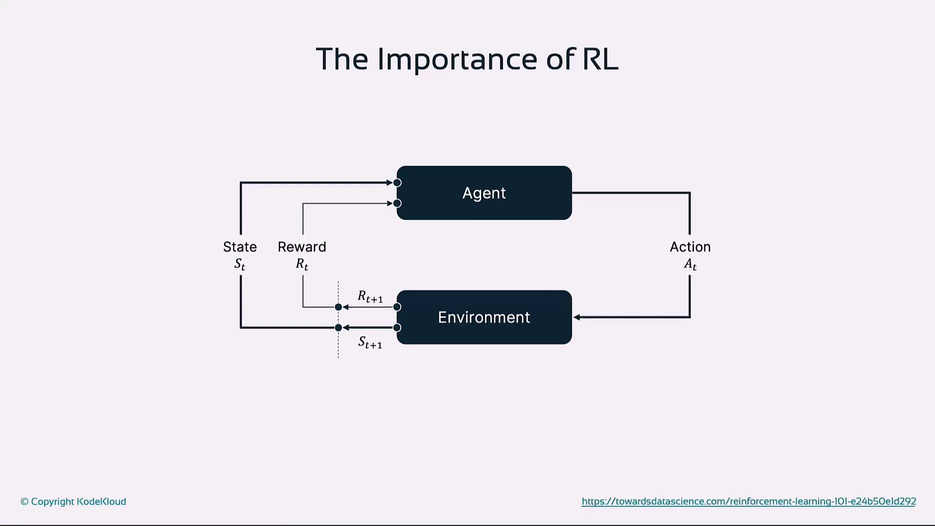
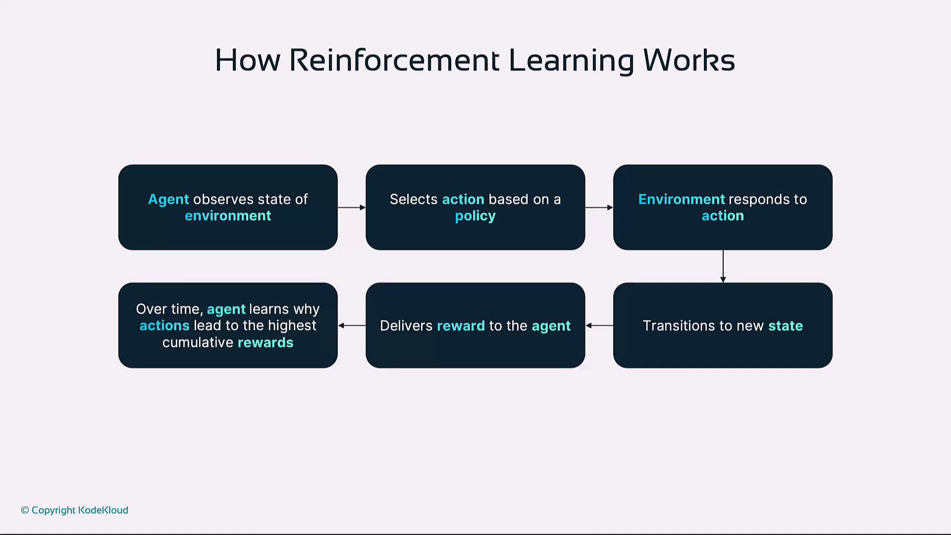
2. How Reinforcement Learning Works
At each time step:- Agent observes state S
- Selects action A using policy π
- Environment returns reward R and next state S′
- Agent updates policy/value estimates to improve future returns
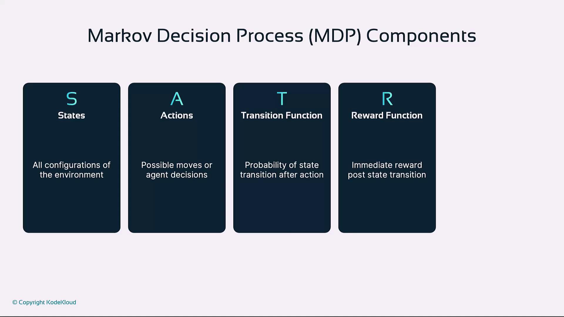
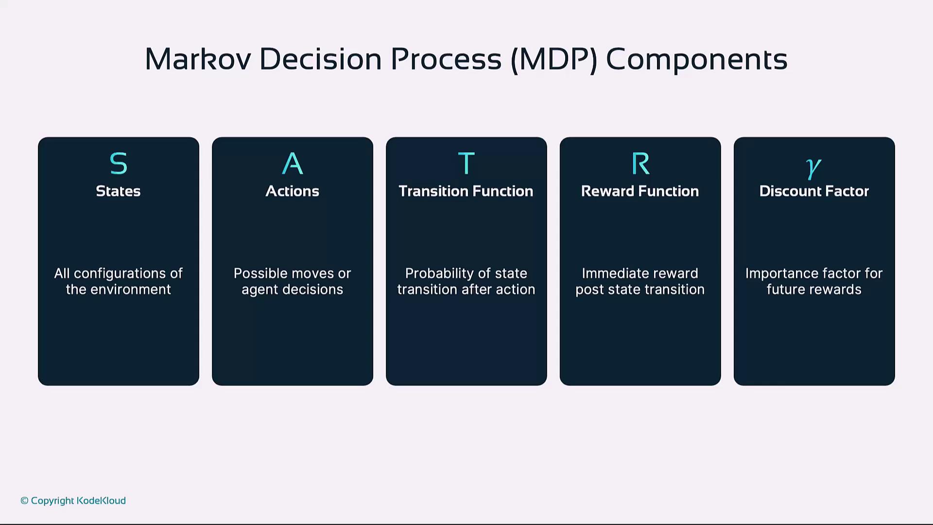
3. Markov Decision Processes
Reinforcement learning problems are often formalized as MDPs, defined by:- States (S): All possible environment configurations
- Actions (A): Moves available to the agent
- Transition Function (T): Probability T(s, a, s′) of moving from state s to s′ after action a
- Reward Function (R): Immediate reward for each transition
- Discount Factor (γ): Importance of future rewards (0 ≤ γ ≤ 1)
MDP assumptions include the Markov property: the next state depends only on the current state and action.
4. Value-Based Methods
Value-based methods focus on estimating the value of states or actions, then choosing actions that maximize expected return.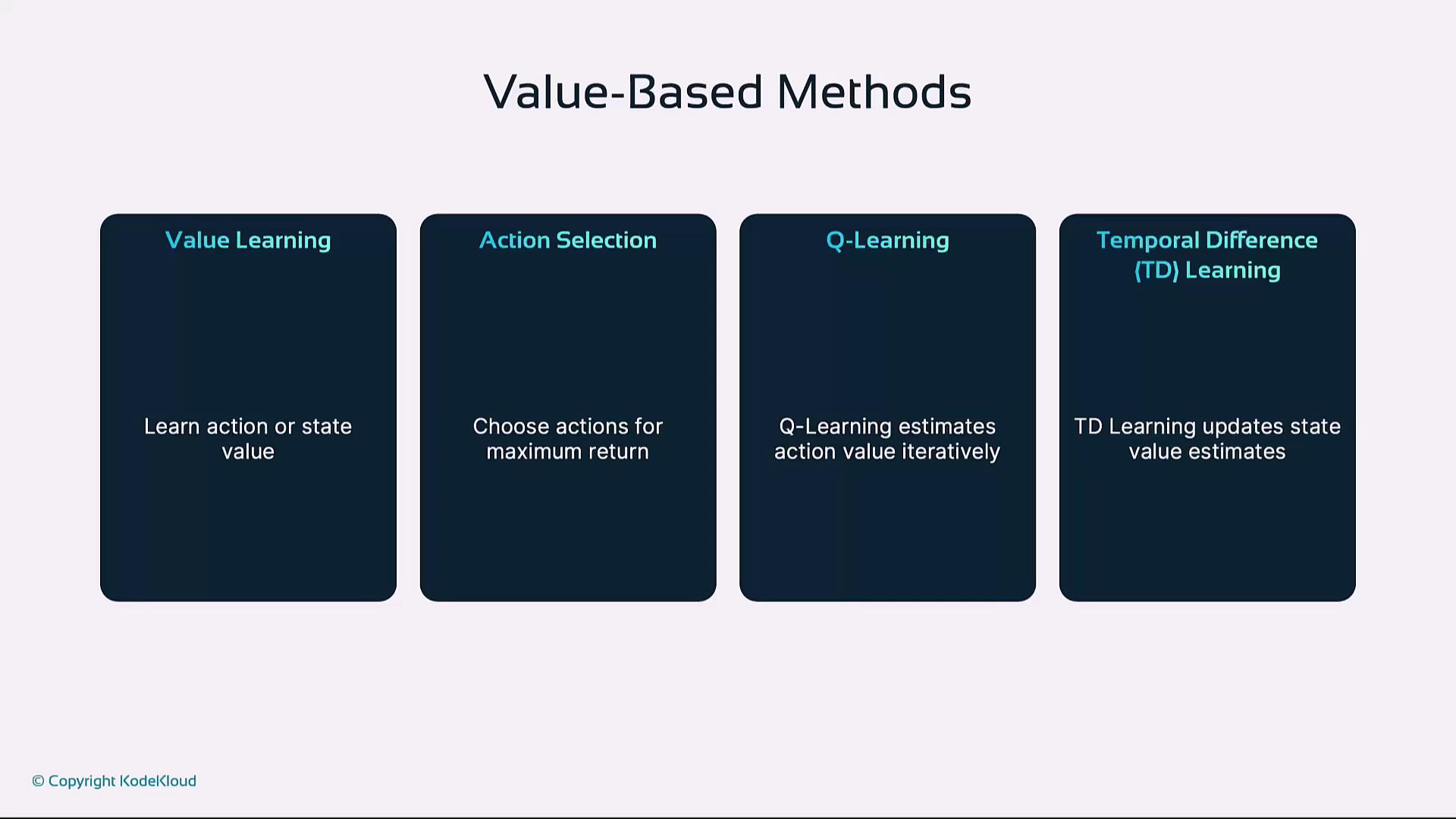
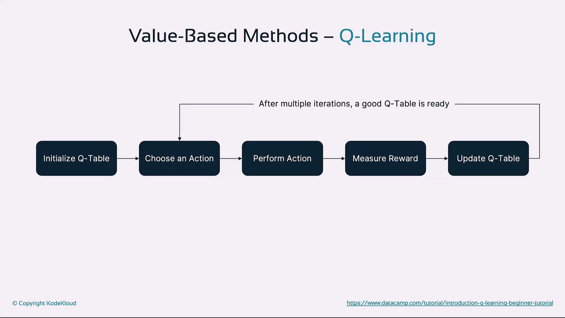
Q-Learning
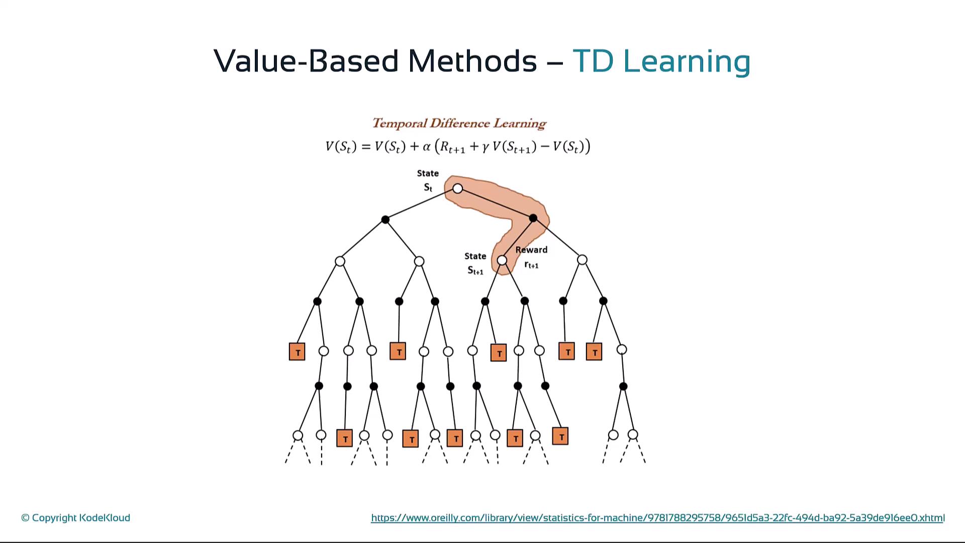
Temporal Difference Learning
5. Policy-Based and Actor-Critic Methods
Policy-Based Methods
Directly optimize the policy π(a|s) without a separate value function. The policy gradient theorem: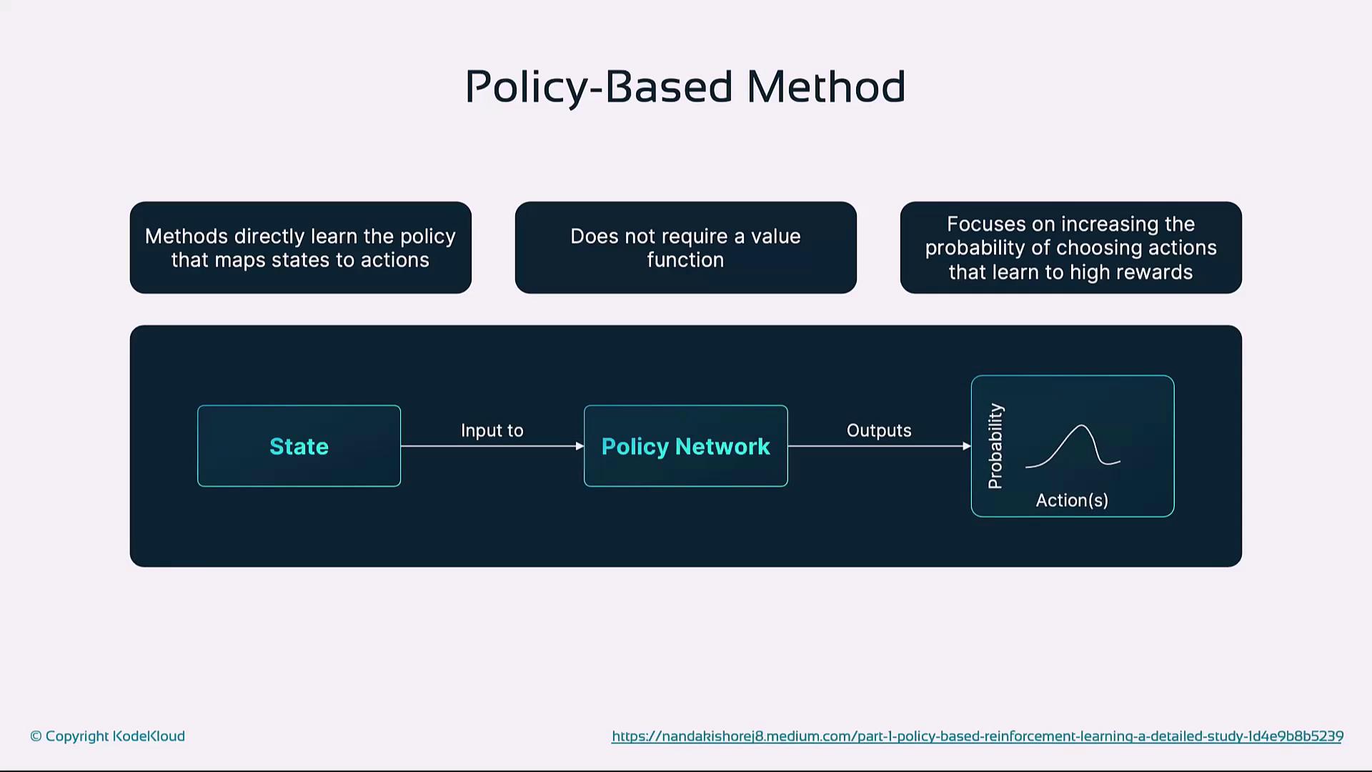
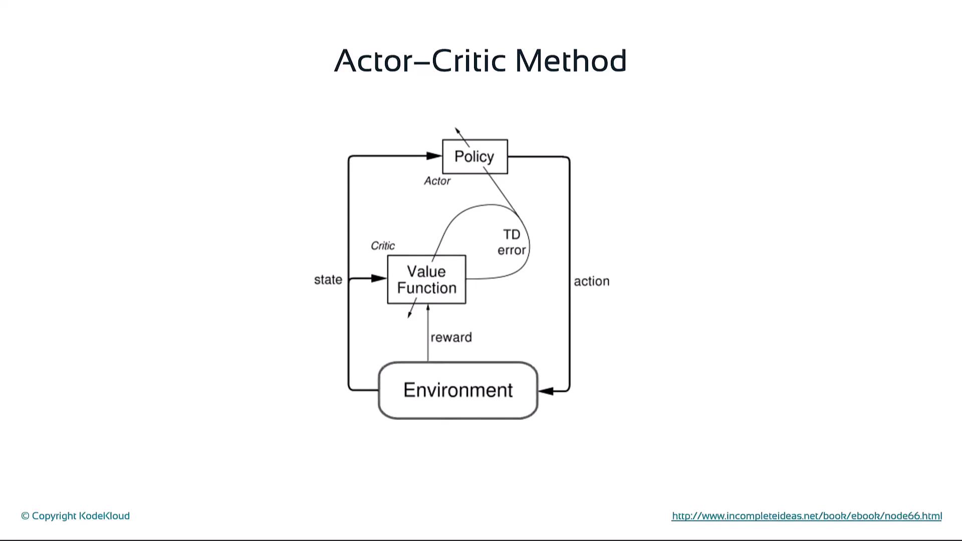
Actor-Critic Methods
Combine policy and value estimation:- Actor: Suggests actions using policy π
- Critic: Evaluates actions via value or TD error
- Critic’s feedback updates both policy parameters θ and value estimates
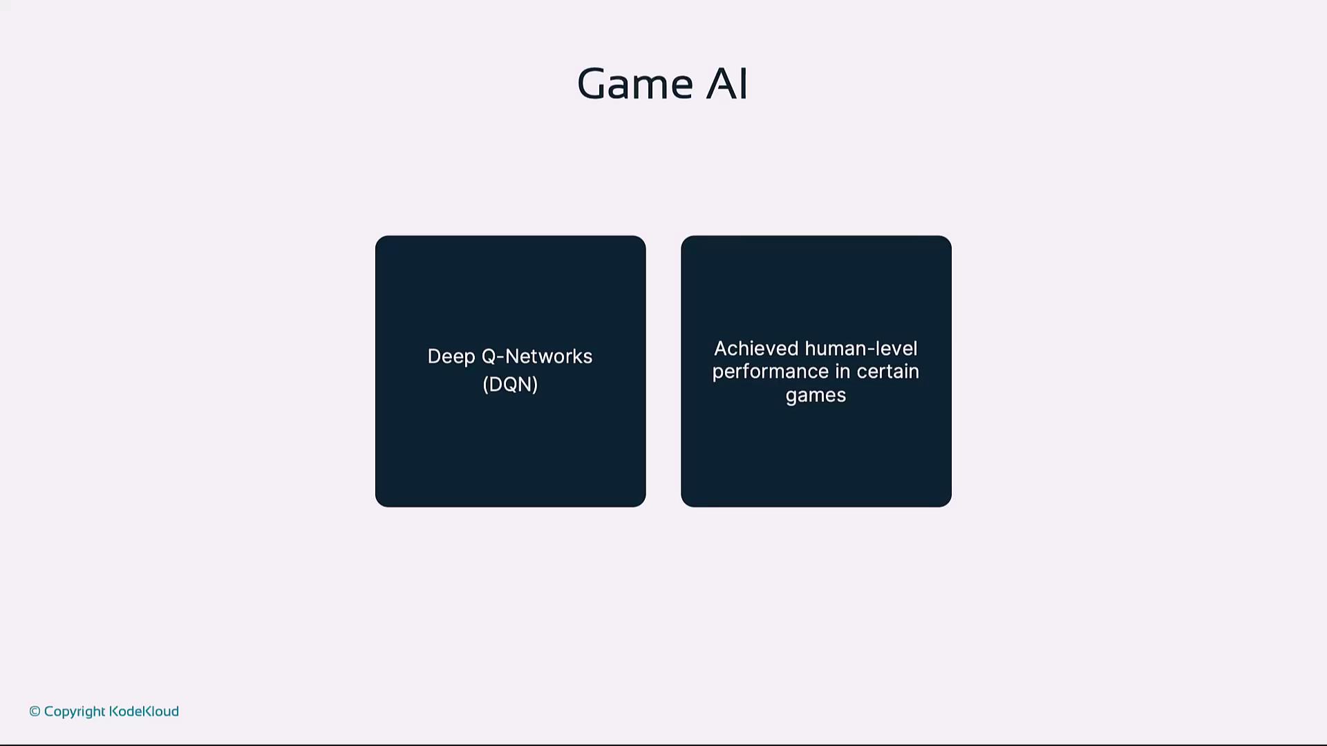
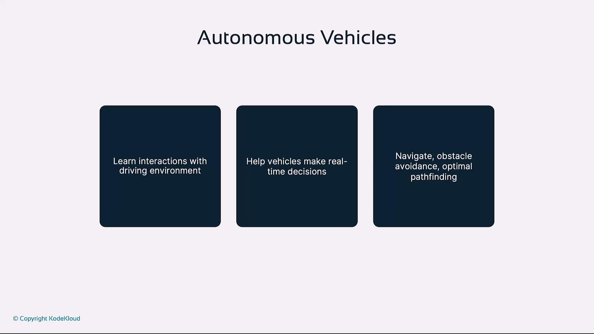
6. Applications of Reinforcement Learning
- Game AI: Deep Q-Networks (DQN) and AlphaGo
- Robotics: Grasping, locomotion, navigation through trial and error
- Autonomous Vehicles: Real-time decisions, obstacle avoidance, path planning
- Healthcare: Personalized treatment planning, dosage optimization, surgical assistance
7. Challenges
- Sample Efficiency: RL often demands vast interactions, increasing compute cost.
- Exploration in Large State Spaces: Finding important states without exhaustive search is hard.

Poorly designed reward functions can lead to unintended or unsafe behaviors. Always validate and test reward shaping thoroughly.
- Reward Shaping: Crafting appropriate rewards is critical to guide learning.

8. Future Directions
- Hybrid Paradigms: Integrate RL with supervised and unsupervised learning to improve efficiency.
- Real-World Deployment: Advance safety, scalability, and robustness for finance, logistics, and healthcare.