Building and Training a model

Now that we have an understanding of neural networks and their role in PyTorch, we will walk through building and training a neural network model. In this guide, we cover how to define a neural network using PyTorch, explore model parameters, loss functions, and optimizers, and learn how to train your model effectively.

This is an exciting section where theory meets hands-on implementation.

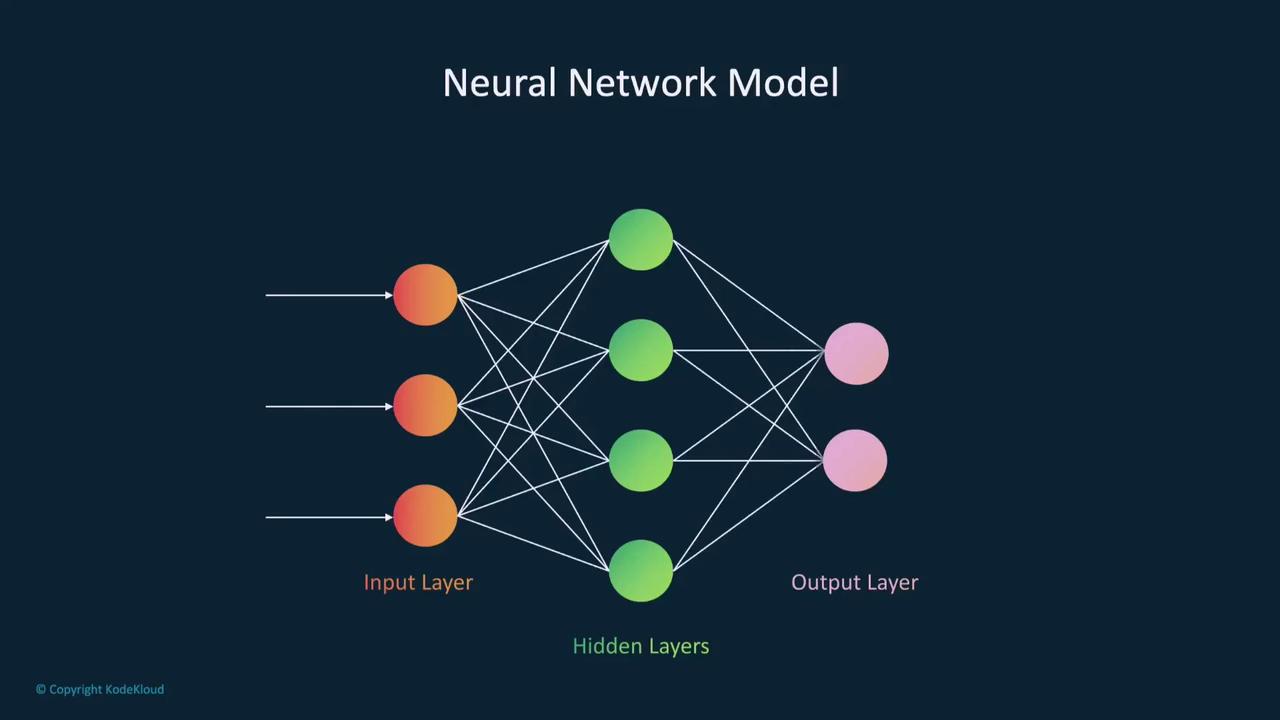
What Is a Model?

A model can be thought of as a blueprint or recipe that makes predictions based on input data. A popular type of model is a neural network, inspired by the human brain's structure and function.

A neural network is composed of layers of neurons, which work together to learn patterns in data. In PyTorch, you create a structure where input data passes through these layers and produces an output—such as identifying objects in an image.

PyTorch streamlines model creation by providing essential tools to define and link layers.

Defining a Neural Network Model in PyTorch

To build a neural network in PyTorch, you create a class that inherits from torch.nn.Module. This class serves as a blueprint that defines the layers and the flow of data through them.

Below is an example of a simple neural network class:

import torch
import torch.nn as nn

# Define the neural network by creating a class
class SimpleNeuralNetwork(nn.Module):
    def __init__(self):
        super(SimpleNeuralNetwork, self).__init__()

        # Define the layers
        self.input_layer = nn.Linear(10, 20)
        self.hidden_layer = nn.Linear(20, 15)
        self.output_layer = nn.Linear(15, 1)

        # Define the activation function
        self.activation = nn.ReLU()

    # Define the forward pass
    def forward(self, x):
        x = self.activation(self.input_layer(x))
        x = self.activation(self.hidden_layer(x))
        x = self.output_layer(x)
        return x

In this class:

• The __init__ method sets up the input, hidden, and output layers, along with the ReLU activation function.
• The forward method dictates how data flows through the network, from the input layer to the final output.

When you create an instance of this class, PyTorch recognizes it as a neural network model automatically.

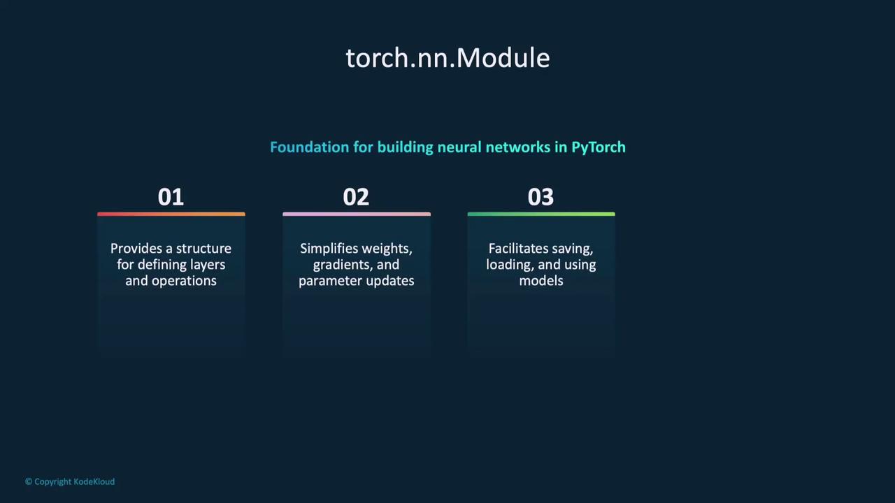
Understanding torch.nn.Module

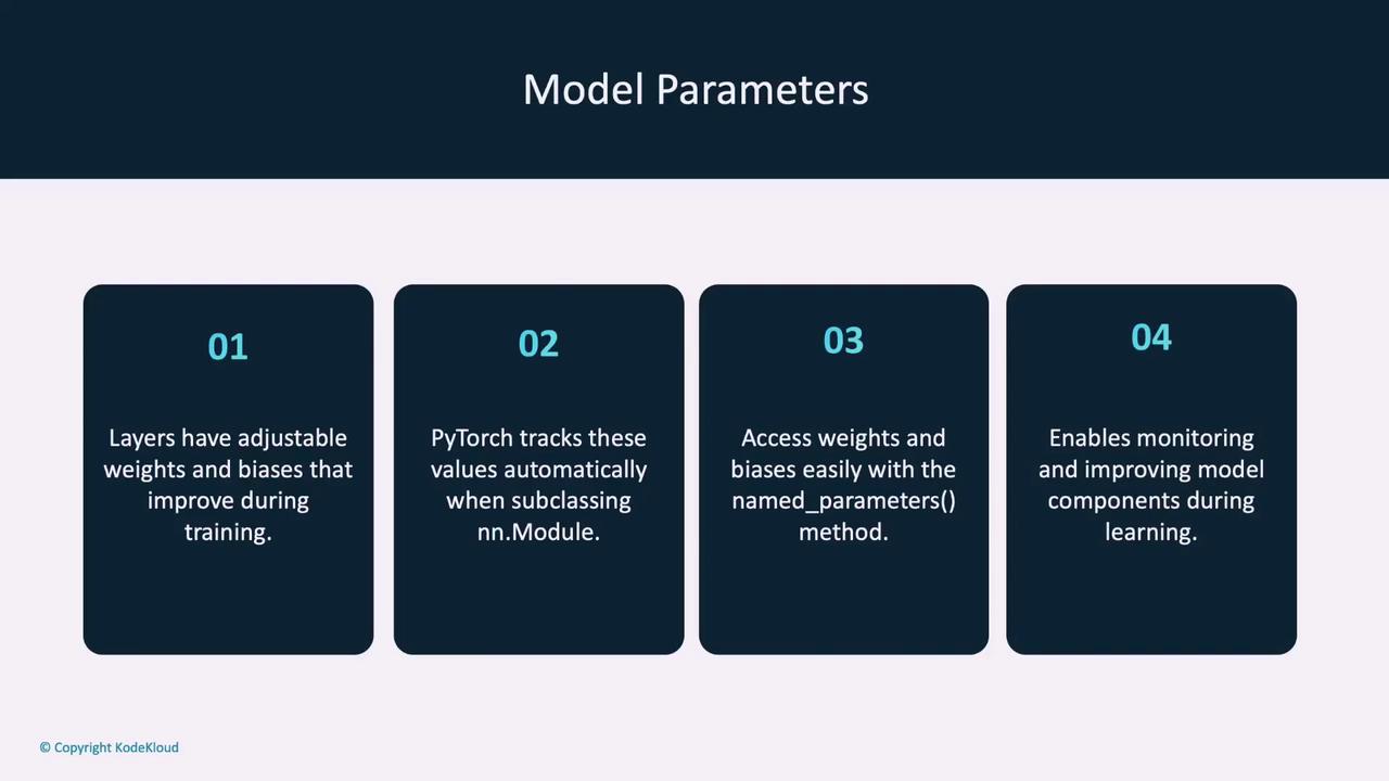
The torch.nn.Module class offers a structured approach for defining layers and operations in your model. By inheriting from this module, you benefit from features such as automatic management of weights, gradients, and parameter updates. This design also simplifies saving, loading, and reusing your model.

In the __init__ function, by defining the layers, you ensure that they are primed to process data seamlessly.

A Quick Overview of Neural Network Layers

When designing a neural network, you have various types of layers at your disposal. Here are some common layer types used in PyTorch:

1. Fully Connected Layer (Dense Layer)

   • Every neuron in one layer is connected to every neuron in the next.
   • Implemented as nn.Linear.

2. Convolutional Layer

   • Ideal for image processing.
   • Uses convolutional filters to extract features such as edges and textures.
   • Implemented as nn.Conv2d.

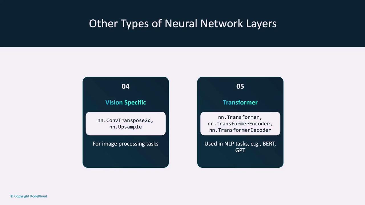
3. Recurrent Layer

   • Suitable for sequential data like time-series or text.
   • Examples include nn.RNN, nn.LSTM, and nn.GRU.

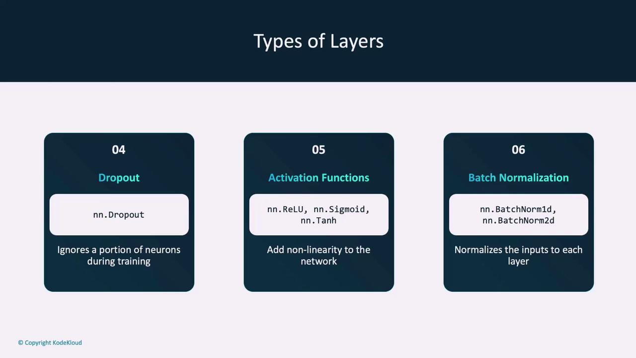
4. Dropout Layer

   • Randomly ignores a portion of neurons during training, helping to prevent overfitting.

5. Activation Functions

   • Introduce non-linearity into the network (e.g., ReLU for hidden layers, sigmoid or softmax for output layers).

6. Batch Normalization

   • Normalizes the outputs of each layer to improve training stability and speed.

Other layers include pooling (MaxPool, AveragePool), padding, and embedding layers (common in NLP tasks). Vision-specific layers, such as transformer layers, are used in advanced image processing and NLP models.

Transformers are widely used in state-of-the-art models like BERT and GPT:

nn.ConvTranspose2d,
nn.Upsample

nn.Transformer,
nn.TransformerEncoder,
nn.TransformerDecoder

The Forward Function

In a PyTorch model, the forward function defines the sequence of operations and transformations that generate a prediction from input data. Essentially, it processes data through each layer and produces an output.

Consider the simplified example below that demonstrates the forward pass:

def forward(self, x):
    x = self.activation(self.input_layer(x))
    x = self.activation(self.hidden_layer(x))
    x = self.output_layer(x)
    return x

This function enables the model to process inputs and generate predictions. Once the class is defined, creating an instance and printing the model structure provides visibility into its layers:

# Create an instance of the model
model = SimpleNeuralNetwork()

# Print the model structure
print(model)

Printing the model displays the input, hidden, and output layers along with their corresponding parameters (weights and biases).

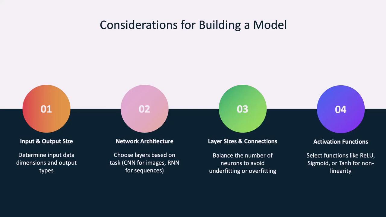
Designing Your Network

When designing your neural network, consider the following factors:

• Output Size: Analyze the dimensions of your input data and determine the desired output (e.g., classification labels versus regression values). This affects the configuration of the first and last layers.
• Network Architecture: Choose the appropriate architecture based on the task. For instance, CNNs are optimal for image data, while RNNs suit sequential data. Experimentation with existing architectures is useful.
• Layers and Connections: Decide the number of neurons and the connectivity between layers. Too few neurons may cause underfitting, whereas too many may lead to overfitting.
• Activation Functions: Select the right activation functions (e.g., ReLU, sigmoid, or tanh) to capture non-linear patterns within your data.

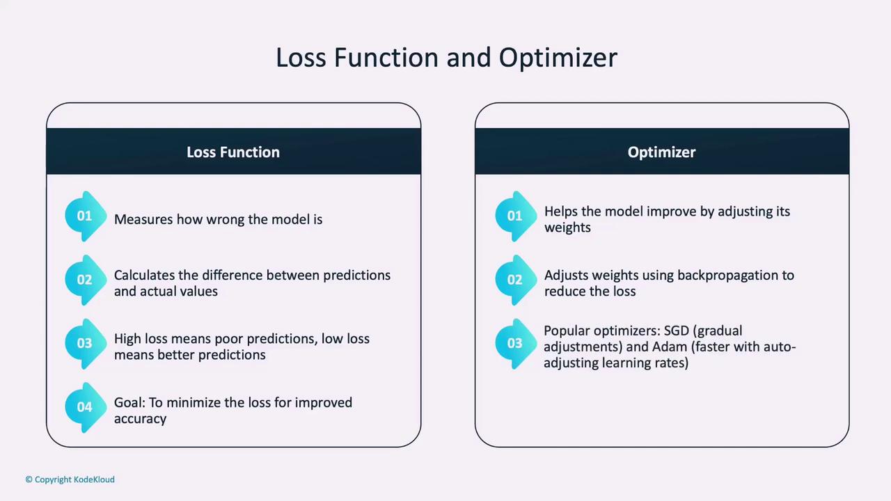
Loss Functions and Optimizers

After designing the model, the next step is training. Training involves optimizing the model's parameters (weights and biases) by reducing the error using loss functions and optimizers.

• Loss Function: This function measures how well the model's predictions match the target values. Common examples include cross-entropy loss for classification tasks and mean squared error (MSE) for regression tasks.
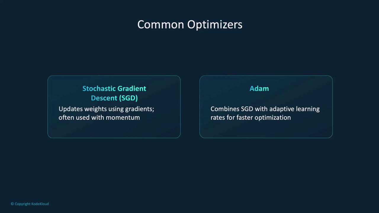
• Optimizer: The optimizer adjusts the model’s parameters to minimize the loss using gradients computed via backpropagation. Popular optimizers include Stochastic Gradient Descent (SGD) and Adam.

Below is an example that defines a loss function and an optimizer for a model:

import torch.optim as optim

criterion = nn.CrossEntropyLoss()
optimizer = optim.SGD(model.parameters(), lr=0.001, momentum=0.9)

Here, criterion is set to cross-entropy loss for classification tasks, and optimizer is configured as SGD with a learning rate of 0.001 and momentum of 0.9. Other loss functions such as Mean Squared Error (MSELoss) and Binary Cross-Entropy (BCELoss) cater to regression and binary classification tasks, respectively.

Common optimizers include:

• Stochastic Gradient Descent (SGD): Updates weights based on gradients, often enhanced with momentum.
• Adam: Combines SGD with adaptive learning rates for improved optimization.

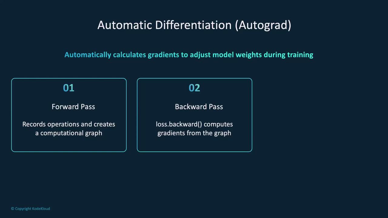
Automatic Differentiation with Autograd

One of PyTorch's standout features is automatic differentiation with Autograd. This mechanism tracks operations performed on Tensors to build a computational graph, which is later used to compute gradients during backpropagation. When you invoke loss.backward(), Autograd calculates the gradients for each parameter, guiding the optimizer in updating the model's weights.

This automated gradient computation simplifies the training process by eliminating the need for manual derivative calculations.

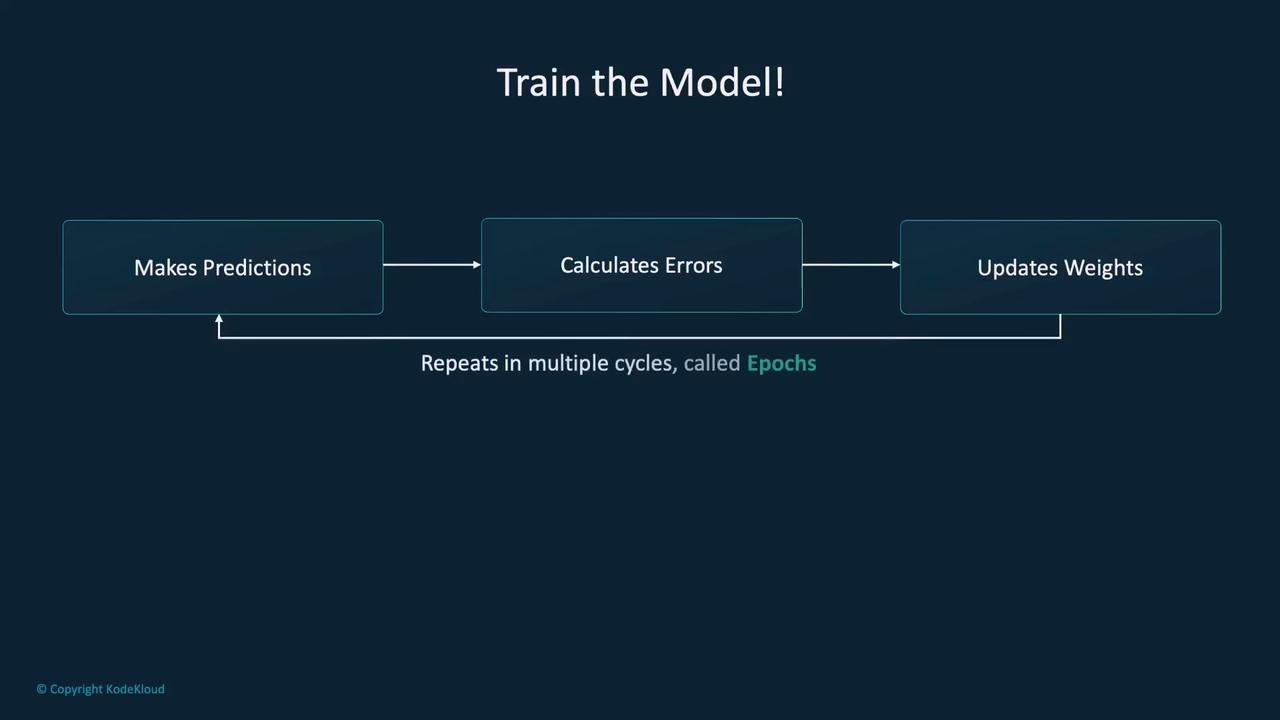
Training the Model

With the neural network, loss function, and optimizer defined, the next step is training the model. Training involves iterating through the dataset over multiple epochs. In each epoch, the model:

• Makes predictions.
• Calculates the loss.
• Computes gradients using backpropagation.
• Updates its weights via the optimizer.

An epoch signifies one complete pass through the training dataset.

Example Training Loop

Below is an example demonstrating a training loop that runs over three epochs:

N_EPOCHS = 3

for epoch in range(N_EPOCHS):  # Loop for 3 epochs
    running_loss = 0.0
    for i, data in enumerate(trainloader, 0):
        # Get the inputs; data is a list of [inputs, labels]
        inputs, labels = data

        # Zero the gradients before backpropagation
        optimizer.zero_grad()

        # Forward pass
        outputs = model(inputs)
        loss = criterion(outputs, labels)

        # Backward pass and optimization
        loss.backward()
        optimizer.step()

        # Accumulate the batch loss
        running_loss += loss.item()

    print(f"Epoch: {epoch} Loss: {running_loss/len(trainloader)}")

In this loop:

• Data is fetched in batches from trainloader.
• Gradients are reset using optimizer.zero_grad().
• A forward pass calculates predictions.
• The loss is then backpropagated, and the optimizer updates the model parameters.
• The average loss for each epoch is printed to monitor training progress.

Incorporating Validation Data

Validating your model during training is essential for ensuring that it generalizes well and does not overfit the training data. Overfitting occurs when the model learns the details and noise in the training dataset too well, resulting in poor performance on unseen data.

Updated Training Loop with Validation

The example below demonstrates a training loop that includes a validation phase:

N_EPOCHS = 3

for epoch in range(N_EPOCHS):  # Loop for 3 epochs
    # Training phase
    training_loss = 0.0
    model.train()  # Set the model to training mode
    for i, data in enumerate(trainloader, 0):
        inputs, labels = data
        optimizer.zero_grad()  # Reset gradients
        outputs = model(inputs)  # Forward pass
        loss = criterion(outputs, labels)  # Compute loss
        loss.backward()  # Backpropagation
        optimizer.step()  # Update parameters
        training_loss += loss.item()

    # Validation phase
    val_loss = 0.0
    model.eval()  # Set the model to evaluation mode
    for i, data in enumerate(valoader, 0):
        inputs, labels = data
        outputs = model(inputs)  # Forward pass
        loss = criterion(outputs, labels)
        val_loss += loss.item()

    print(f"Epoch: {epoch} Train Loss: {training_loss/len(trainloader)} Val Loss: {val_loss/len(valoader)}")

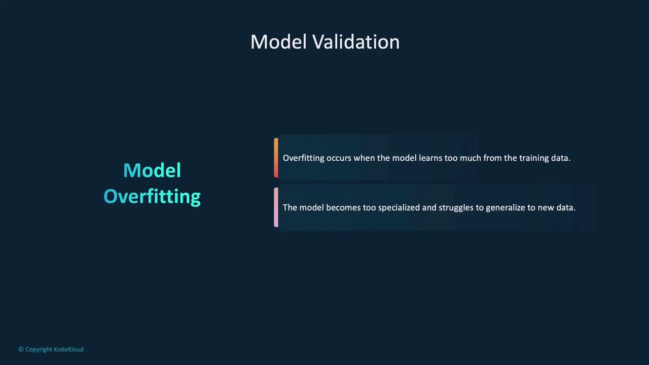
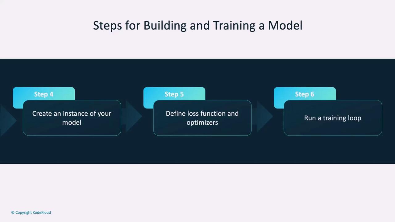
Recap of the Steps

1. Define the Model:

   • Create a class that inherits from torch.nn.Module.
   • Define the network layers in the __init__ method.
   • Specify the data flow in the forward method.

2. Set Up the Training Environment:

   • Initialize the model.
   • Define a loss function to quantify errors.
   • Set up an optimizer to adjust model parameters.

3. Implement the Training Loop:

   • Iterate through batches for several epochs.
   • Perform forward passes, compute the loss, backpropagate, and update weights.
   • Optionally incorporate validation to monitor generalization.

Conclusion

In this article, we have covered:

• How to build a neural network in PyTorch by defining a class that inherits from torch.nn.Module.
• How to design the network structure, including layer definitions and the forward pass.
• The importance of loss functions and optimizers in training.
• How to implement a training loop that incorporates validation to combat overfitting.

This foundational knowledge paves the way for exploring more advanced topics and practical demonstrations of neural networks in action.