Demo Introduction to Transformations

Welcome to this technical lesson on PyTorch image transformations. In this guide, you'll learn how to utilize PyTorch transformations for data preprocessing and augmentation to boost model performance and efficiency. PyTorch’s TorchVision library offers a comprehensive set of transformation classes that convert raw image data into formats that are optimized for model training and can augment your dataset by adding variability.

Below, we demonstrate various transformation techniques—including resizing, random horizontal flips, tensor conversion, normalization, random cropping, photometric distortions, random resizing, and building transformation pipelines with Compose—each explained with its corresponding code snippet.

Helper Function to Display Images

We begin by defining a helper function to visualize the original image alongside its transformed version. This function is essential for comparing the effects of different transformations in real time.

import matplotlib.pyplot as plt

def display_images(original_image, new_image=None, new_image_name=None):
    """
    Helper function to display images.
    If a new image is provided, shows them side by side.
    """
    if new_image is not None:
        fig, axes = plt.subplots(1, 2, figsize=(10, 5))
        axes[0].imshow(original_image)
        axes[0].axis('on')  # Display axis for context
        axes[0].set_title('Original Image')
        axes[1].imshow(new_image)
        axes[1].axis('on')
        axes[1].set_title(new_image_name)
    else:
        plt.figure(figsize=(10, 5))
        plt.imshow(original_image)
        plt.axis('on')
    plt.show()

You can now use this function to visually compare the before and after images for every transformation applied.

Loading an Image with Pillow and PyTorch Transforms

In this section, we load an image of a cat using the Pillow library while utilizing both version 2 and version 1 of the transform APIs.

from torchvision.transforms import v2
from torchvision import transforms
from PIL import Image

# Load the image using Pillow
original_image = Image.open('images/cat/cat-1.jpg')
print(original_image)

# Display the loaded image
display_images(original_image=original_image)

Resizing an Image

Resizing ensures consistent image dimensions across your dataset. In the example below, we resize the image to 50×25 pixels using the PyTorch v2 API.

# Using v2 Resize transform to set image dimensions to 50x25 pixels
resize_transform = v2.Resize((50, 25))
resized_image = resize_transform(original_image)

# Display the resized image
display_images(original_image=original_image, new_image=resized_image, new_image_name="Resized Image")

For those who prefer the v1 API, the same operation can be implemented as follows:

# Using v1 transforms.Resize for the identical operation
resize_transform = transforms.Resize((50, 25))
resized_image = resize_transform(original_image)
display_images(original_image=original_image, new_image=resized_image, new_image_name="Resized Image")

Random Horizontal Flip

Random horizontal flips augment your dataset by mirroring images randomly. In this demonstration, we set the flip probability to 100% (p=1) for clarity.

# Random horizontal flip with 100% probability
rh_transform = v2.RandomHorizontalFlip(p=1)
rhf_image = rh_transform(original_image)
display_images(original_image=original_image, new_image=rhf_image, new_image_name="Random Horizontal Flip")

Converting Images to Tensors

Before feeding images into a PyTorch model, they must be converted into tensors. This transformation scales pixel intensity values appropriately for model consumption.

from torchvision.transforms import ToTensor

# Convert image to tensor
tensor_transform = ToTensor()
tensor_image = tensor_transform(original_image)

print(f"Original Image: {original_image}")
print(f"Tensor Image: \n{tensor_image}")

Normalizing Tensor Images

Normalization adjusts pixel intensity values to a standardized range, which is crucial for faster model convergence. Here, we normalize the tensor with a mean and standard deviation of (0.5, 0.5, 0.5).

# Normalize the tensor image
normalize_transform = v2.Normalize((0.5, 0.5, 0.5), (0.5, 0.5, 0.5))
normalized_image = normalize_transform(tensor_image)

# Display normalized tensor along with the original tensor for comparison
print(normalized_image)
print(tensor_image)

Random Cropping

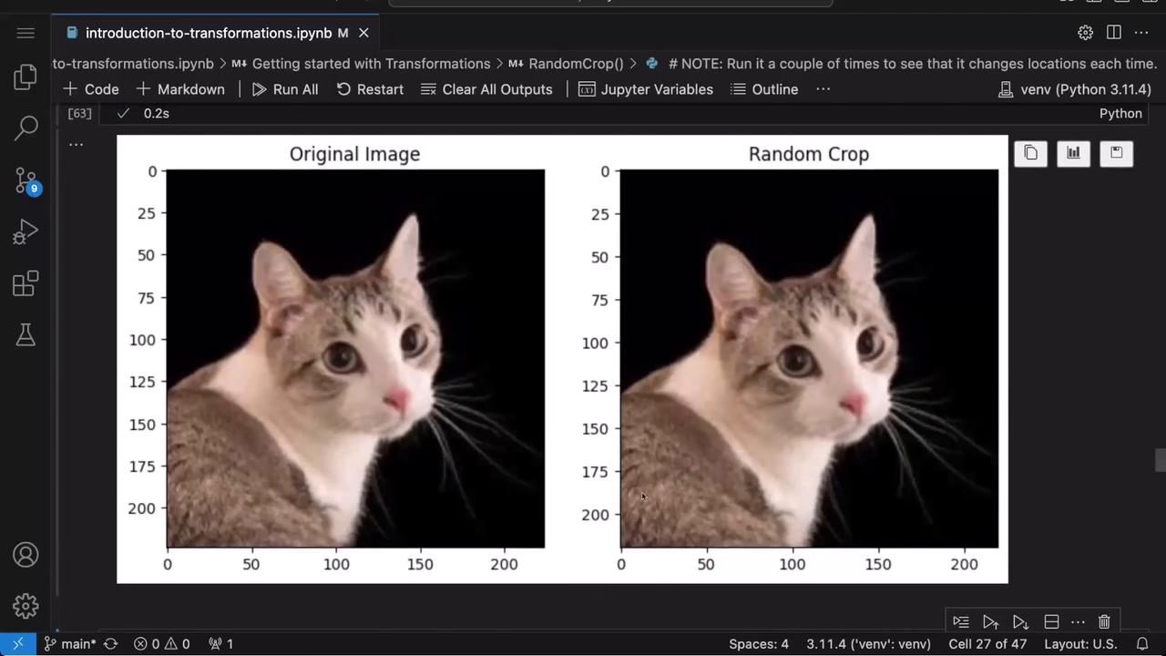
Random cropping extracts a fixed-size region from an image, which is useful for data augmentation. In this example, we extract a 100×100 pixel patch.

# Randomly crop a 100x100 pixel region from the image
rc_transform = v2.RandomCrop(size=(100, 100))
rc_image = rc_transform(original_image)
display_images(original_image=original_image, new_image=rc_image, new_image_name="Random Crop")

Running the transformation multiple times yields crops from different parts of the image.

Random Photometric Distortion

Photometric distortion augments images by adjusting brightness, contrast, saturation, and hue. This increases the variation in lighting conditions, helping to improve model generalization.

# Create a photometric distortion transform with specified parameter ranges
rpd_transform = v2.RandomPhotometricDistort(
    brightness=(0.875, 1.125),
    contrast=(0.5, 1.5),
    saturation=(0.5, 1.5),
    hue=(-0.05, 0.05),
    p=1
)

# Apply photometric distortion
rpd_image = rpd_transform(original_image)
display_images(original_image=original_image, new_image=rpd_image, new_image_name="Random Photometric Distort")

Random Resize

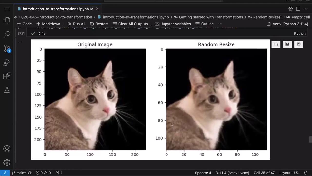
Random resizing applies variable scaling to images, introducing additional diversity into the dataset. Here, the image is randomly resized to a pixel size between 100 and 200.

# Randomly resize the image between 100 and 200 pixels
rr_transform = v2.RandomResize(min_size=100, max_size=200)
rr_image = rr_transform(original_image)
display_images(original_image=original_image, new_image=rr_image, new_image_name="Random Resize")

Building Transformation Pipelines with Compose

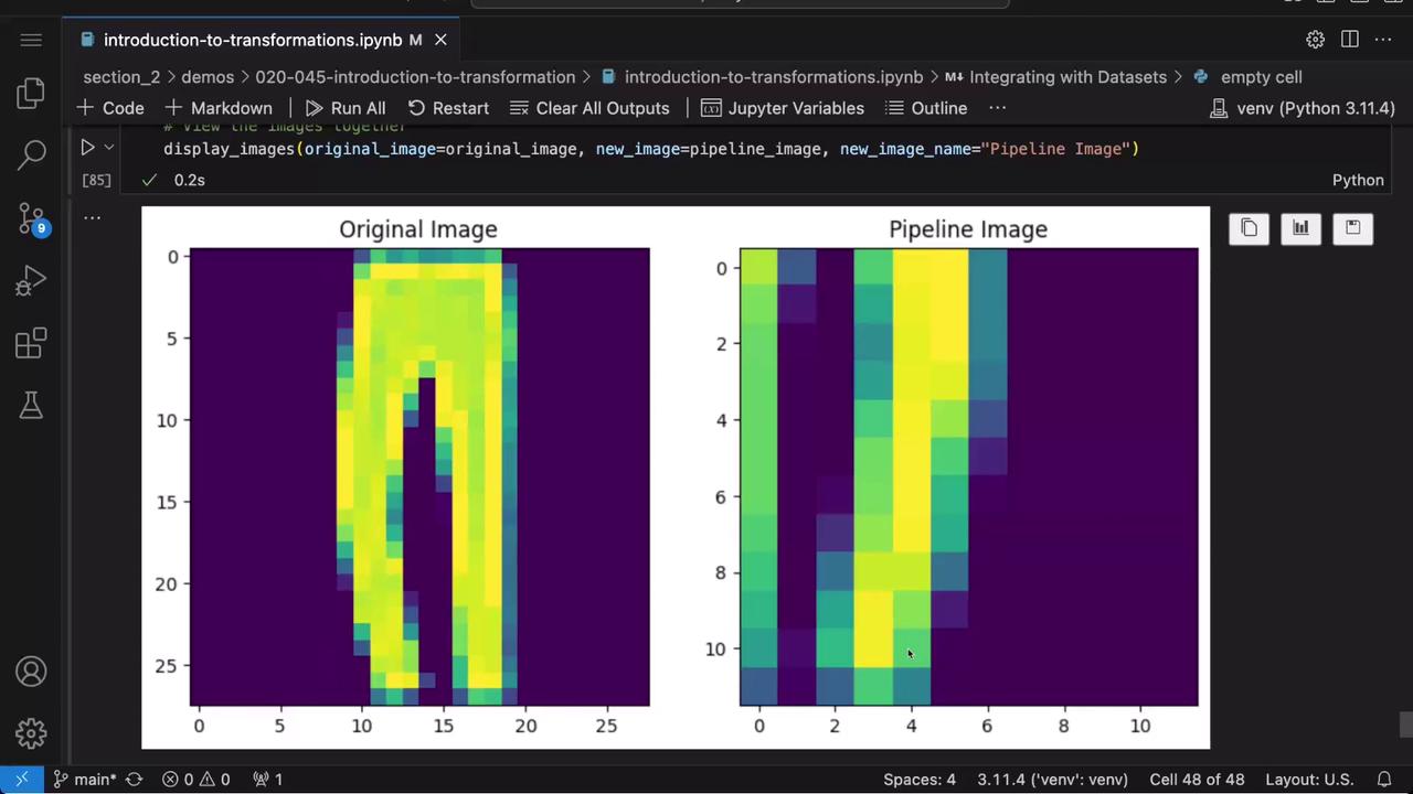
The Compose class enables you to chain multiple transformations together into a single, streamlined pipeline. This approach ensures that every image undergoes the same sequence of augmentations.

# Build a transformation pipeline combining several augmentations
transforms_pipeline = v2.Compose([
    v2.RandomCrop(size=(100, 100)),
    v2.RandomPhotometricDistort(
        brightness=(0.875, 1.125),
        contrast=(0.5, 1.5),
        saturation=(0.5, 1.5),
        hue=(-0.05, 0.05),
        p=1,
    ),
    v2.RandomResize(min_size=75, max_size=150),
    v2.RandomHorizontalFlip(p=1)
])

# Apply the pipeline to the original image
pipeline_image = transforms_pipeline(original_image)

After applying the pipeline, you can view the transformed image as shown below:

display_images(original_image=original_image, new_image=pipeline_image, new_image_name="Pipeline Image")

Applying Transformations to a Dataset

Next, we integrate a transformation pipeline with a real dataset: the Fashion MNIST dataset from TorchVision.

import torchvision.datasets

# Create a FashionMNIST dataset without any transformation
original_image_dataset = torchvision.datasets.FashionMNIST(root='./fashion', train=False, download=True)

# Retrieve and display an image from the dataset
original_image, label = original_image_dataset[2]
display_images(original_image=original_image)

Now, we define a transformation pipeline tailored to the smaller dimensions of Fashion MNIST images:

# Construct a pipeline tailored to Fashion MNIST image size
transforms_pipeline = v2.Compose([
    v2.RandomCrop(size=(15, 15)),
    v2.RandomPhotometricDistort(
        brightness=(0.875, 1.125),
        contrast=(0.5, 1.5),
        saturation=(0.5, 1.5),
        hue=(-0.05, 0.05),
        p=1
    ),
    v2.RandomResize(min_size=10, max_size=15),
    v2.RandomHorizontalFlip(p=1)
])

You can integrate these transformations into the dataset by passing the pipeline as the transform argument:

# Create a new dataset where each image is augmented by the pipeline
transformed_image_dataset = torchvision.datasets.FashionMNIST(
    root='./fashion', train=False, download=True, transform=transforms_pipeline
)

# Retrieve a transformed image and display it alongside the original
transformed_image, label = transformed_image_dataset[2]
display_images(original_image=original_image, new_image=transformed_image, new_image_name="Transformed Fashion MNIST Image")

Conclusion

In this lesson, we explored a variety of image transformation techniques using PyTorch’s TorchVision library. We covered resizing, flipping, cropping, photometric adjustments, normalization, and composing pipelines—all critical steps for effective image preprocessing and data augmentation. These techniques not only standardize your dataset but also improve model robustness and performance. Experiment with these transformations to optimize the augmentation strategies for your projects.

Thank you for following along, and happy coding!