Backpropagation in Neural Networks

Welcome — Alan Chapman from KodeKloud. In this lesson we unpack how neural networks learn from their mistakes using the chain rule and gradient descent. You’ll see a concrete, step-by-step example that connects calculus (derivatives) to the weight updates that improve predictions.

The image features a woman presenting with the text "Mathematics for Computing" and "Backpropagation and Chain Rule" on a purple background with a dotted pattern.

Overview

Backpropagation: the algorithm for computing gradients of the loss w.r.t. each weight by propagating error backward through the network.
Chain rule: the calculus tool that decomposes derivatives of composite functions into products of simpler derivatives.
Gradient descent: the optimization step that uses gradients to update weights and reduce error.

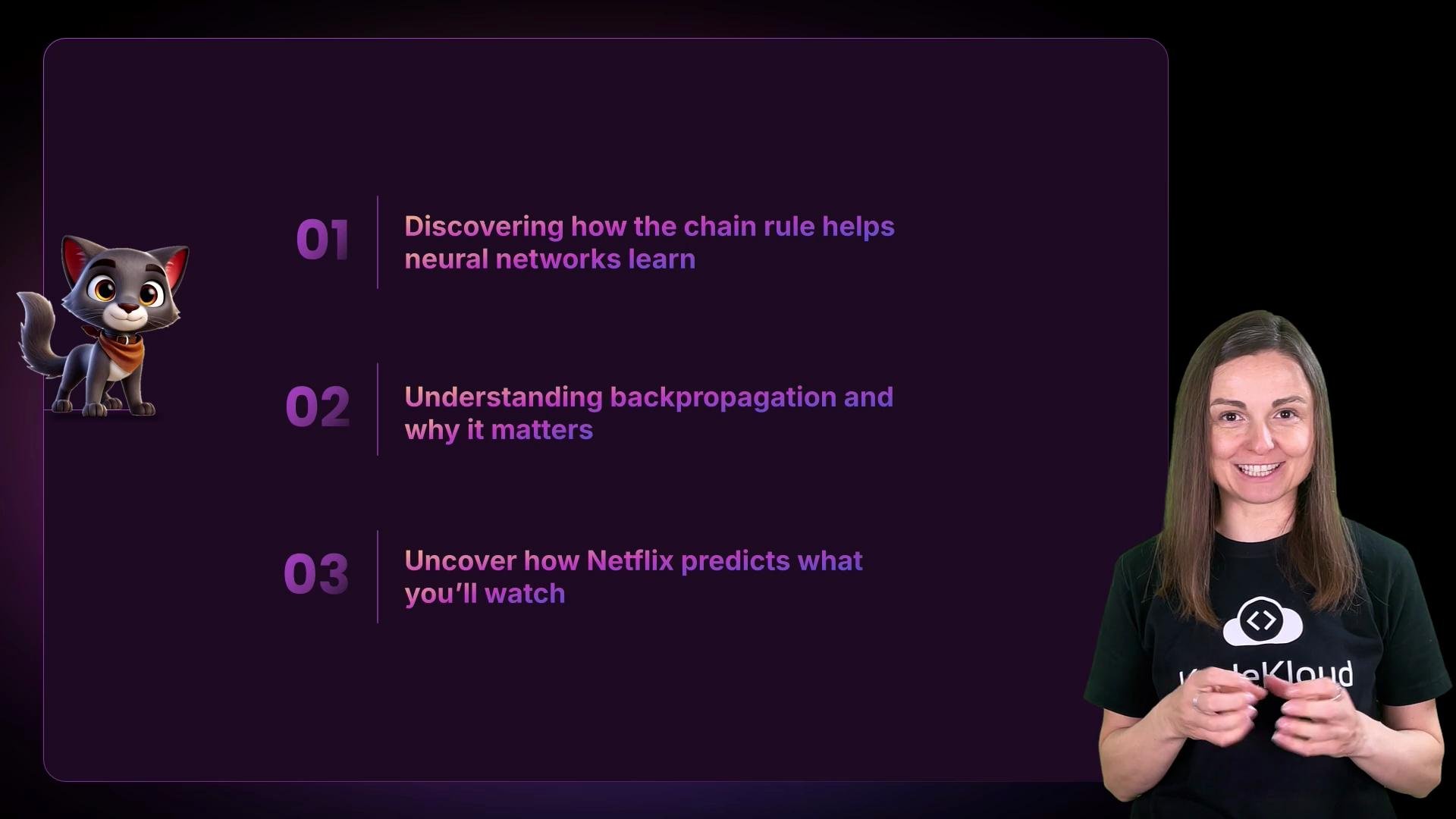
Why this matters (real-world intuition): recommendations (e.g., Netflix) rely on models that continuously adjust internal weights as they observe user interactions — the same calculus principles power that adaptation.

The image features a list of three topics about neural networks and prediction, alongside a cartoon dog and a person wearing a "KodeKloud" shirt.

Example: How Netflix learns your taste When you first sign up, recommendations are noisy. As you interact (watch, rate, skip), the system computes prediction errors and adjusts its parameters so future suggestions better match your preferences.

The image shows a woman standing next to a screen displaying a Netflix interface with various TV shows and movies. The text "How does Netflix know?" is written on the top left.

Neural network anatomy (simple)

Input layer: receives features (e.g., encoded genre, setting).
Hidden layer(s): transform inputs and extract patterns.
Output layer: yields final prediction (e.g., probability of watching a suggested show).
Weights: connections between nodes that determine importance of each input.

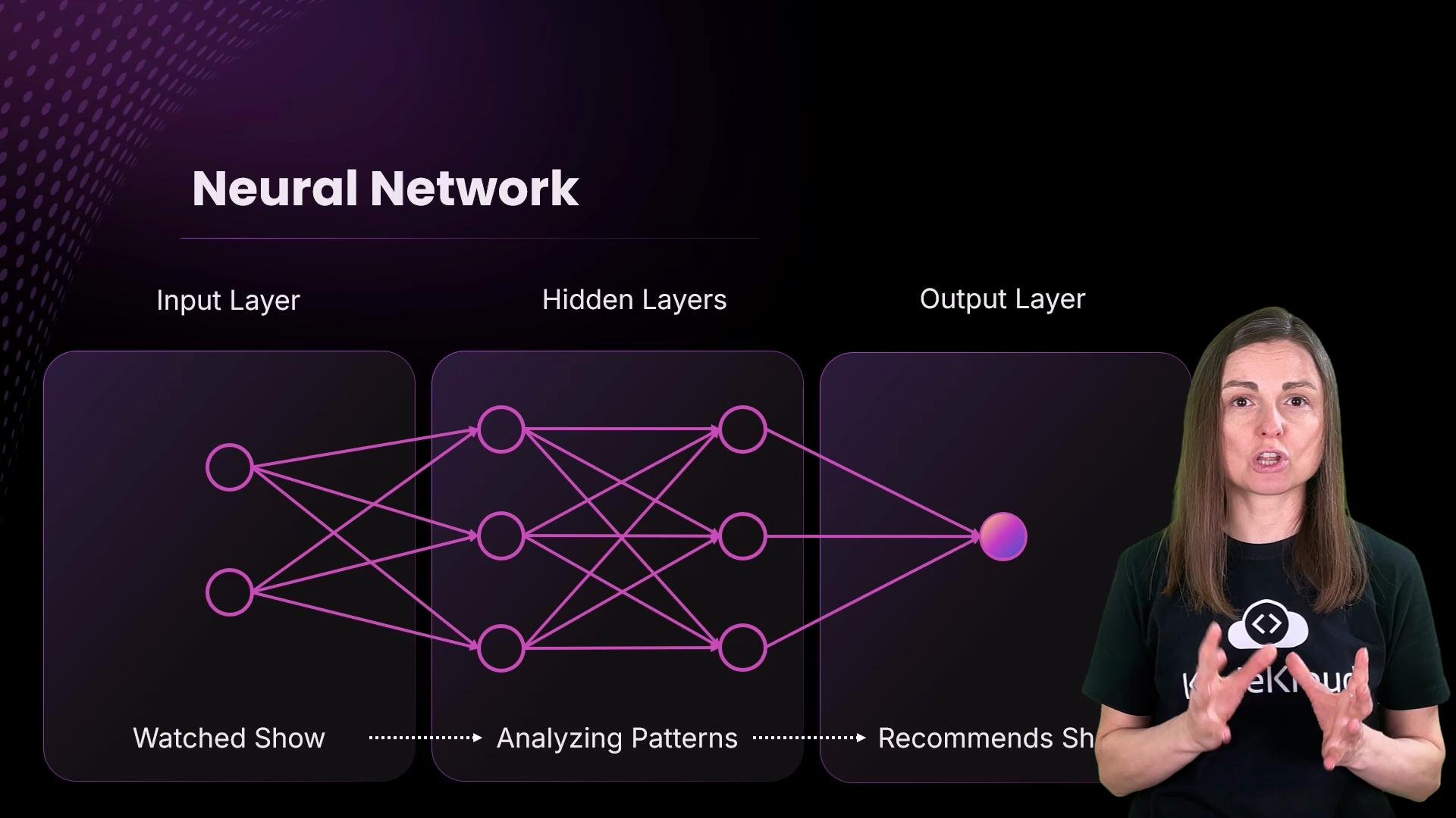
Table — Common components and purpose

Component	Purpose	Example
Input layer	Accepts feature values	`genre`, `setting`
Hidden layer	Learns intermediate features	single neuron for illustration
Output layer	Produces probability or label	probability of watching “Heartstopper”
Weights	Parameters updated during training	`w1`, `w2`
Loss function	Measures prediction error	`0.5*(y - t)^2`

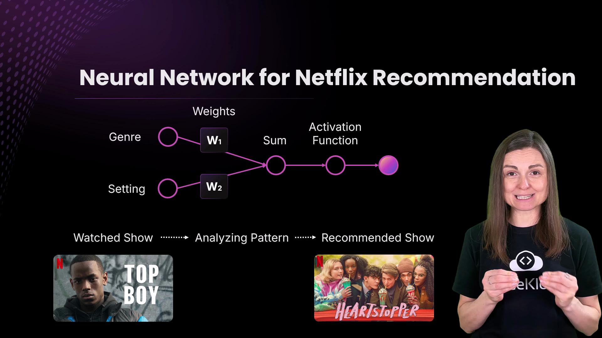
The image shows a diagram of a neural network with input, hidden, and output layers, illustrating the process from "Watched Show" to "Recommends Show." A person is standing beside the diagram, explaining it.

Roles typically involved in building recommendation systems

Machine learning engineers: implement and train models.
Data scientists: analyze and prepare feature data.
AI researchers: design novel architectures and optimization techniques.
Software engineers (AI-focused): integrate models into products.

Table — Roles and responsibilities

Role	Typical responsibilities
Machine learning engineer	Train, validate, deploy models
Data scientist	Feature engineering, experiments
AI researcher	New algorithms, theoretical work
Software engineer (AI)	Product integration, latency/perf

Simplifying to a tiny model We’ll analyze a toy network with:

Two inputs: x1 (genre), x2 (setting)
One hidden neuron (for clarity) and a sigmoid activation at the output
Output y = sigmoid(s), where s = x1w1 + x2w2

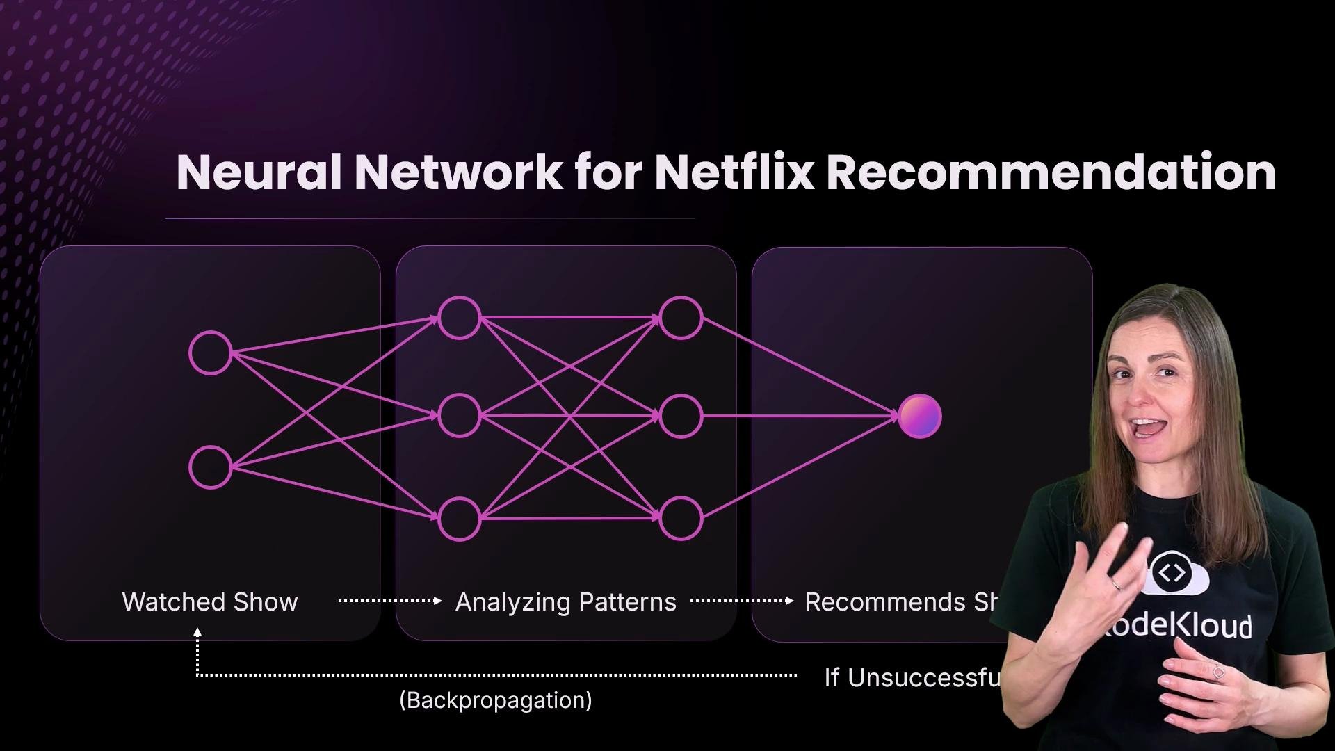
The image illustrates a neural network process for Netflix recommendations, showing stages from watched shows to recommendation and backpropagation. A person stands on the right, wearing a "KodeKloud" t-shirt.

Notation and forward pass

Inputs: x1, x2
Weights: w1, w2
Weighted sum: s = x1w1 + x2w2
Activation (sigmoid): y = sigmoid(s) = 1 / (1 + exp(-s))

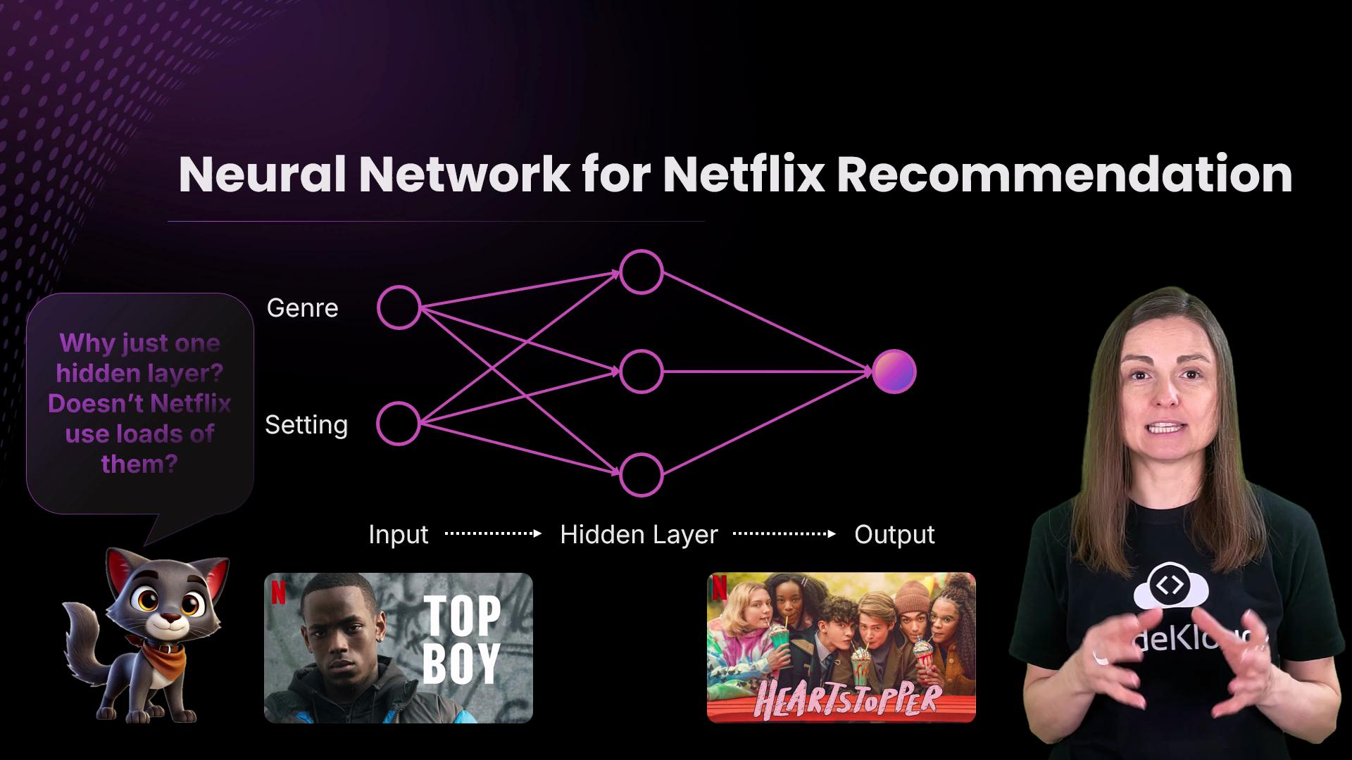
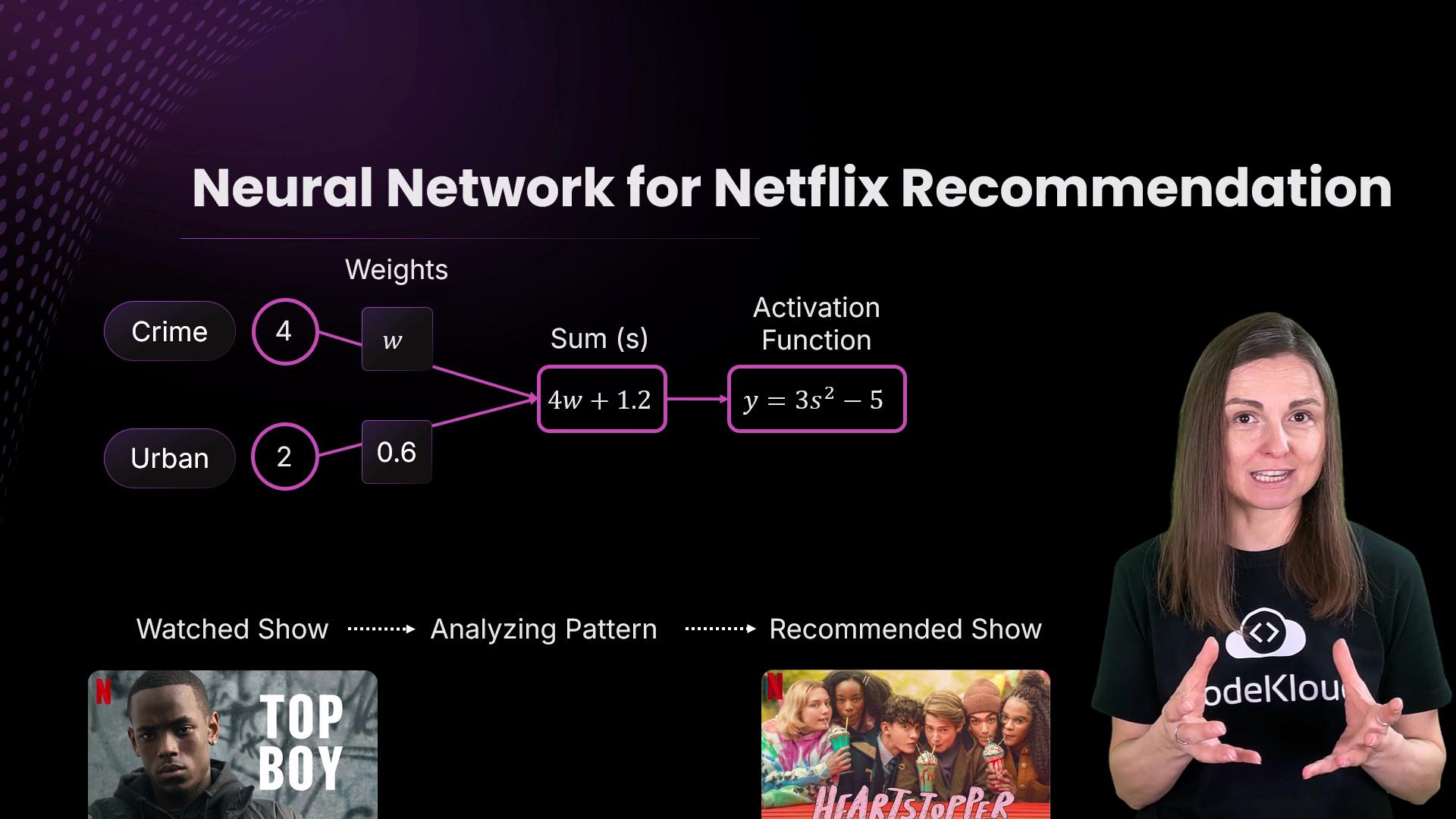
The image illustrates a neural network model for Netflix recommendations, showing inputs as genre and setting, a hidden layer, and outputs with TV show examples. A person is explaining the concept alongside a cartoon cat asking a question about hidden layers.

Concrete numeric example (step-by-step) Given:

x1 = 4.0 (encoded genre)
x2 = 2.0 (encoded setting)
initial weights: w1 = 0.2, w2 = 0.6

Compute s and y:

# python
import math

x1, x2 = 4.0, 2.0
w1, w2 = 0.2, 0.6

s = x1*w1 + x2*w2  # 2.0
y = 1 / (1 + math.exp(-s))  # sigmoid(s)

s, y

Result: s = 2.0, y ≈ 0.8808 (an 88% predicted probability of watching “Heartstopper”).

The image illustrates a neural network for Netflix recommendations, showing how genre and setting are weighted to recommend shows, with examples of "Top Boy" and "Heartstopper." A person stands to the right explaining the concept.

Backpropagation: computing gradients with the chain rule Suppose the observed target is t = 0.65. The model overpredicted, so we compute how to change weights to reduce the error. We want dy/dw1. Since y depends on s and s depends on w1, use the chain rule:

dy/dw1 = (dy/ds) * (ds/dw1)

For the sigmoid:

dy/ds = y * (1 - y)

From s = x1w1 + x2w2:

ds/dw1 = x1

Therefore:

dy/dw1 = x1 * y * (1 - y)

Calculate numerically:

# python
x1 = 4.0
s = 2.0
y = 1 / (1 + math.exp(-s))  # ≈ 0.8807970779778823

dy_ds = y * (1 - y)  # ≈ 0.1050
ds_dw1 = x1  # 4.0

dy_dw1 = dy_ds * ds_dw1  # ≈ 0.420
dy_dw1

So dy/dw1 ≈ 0.420: this is the sensitivity of the output to changes in w1. Loss function and gradient for weight update Use squared-error loss: L = 0.5 * (y - t)^2. Then:

dL/dy = (y - t)
dL/dw1 = dL/dy * dy/dw1 = (y - t) * dy/dw1

Numerically:

error = y - t ≈ 0.8808 - 0.65 = 0.2308
dL/dw1 ≈ 0.2308 * 0.420 ≈ 0.0969

Gradient descent update with learning rate alpha:

# python
alpha = 0.1
error = y - 0.65
dL_dw1 = error * dy_dw1
w1_new = w1 - alpha * dL_dw1
w1_new

This slightly reduces w1 because the model was overpredicting. The same approach computes dL/dw2 using ds/dw2 = x2 and updates w2 accordingly.

The image illustrates a neural network process for Netflix recommendations, showing weights and activation functions, alongside a person explaining the concept.

Callout: key intuition

Backpropagation combines local derivatives: compute how a small change to a weight affects the node output, then multiply by how that output affects the loss. In practice this scales to many layers by repeatedly applying the chain rule from output back to inputs.

Practical note about training

Choose the learning rate (alpha) carefully. Too large -> divergence/overshooting; too small -> very slow learning. Also, scale and normalize inputs for stable training.

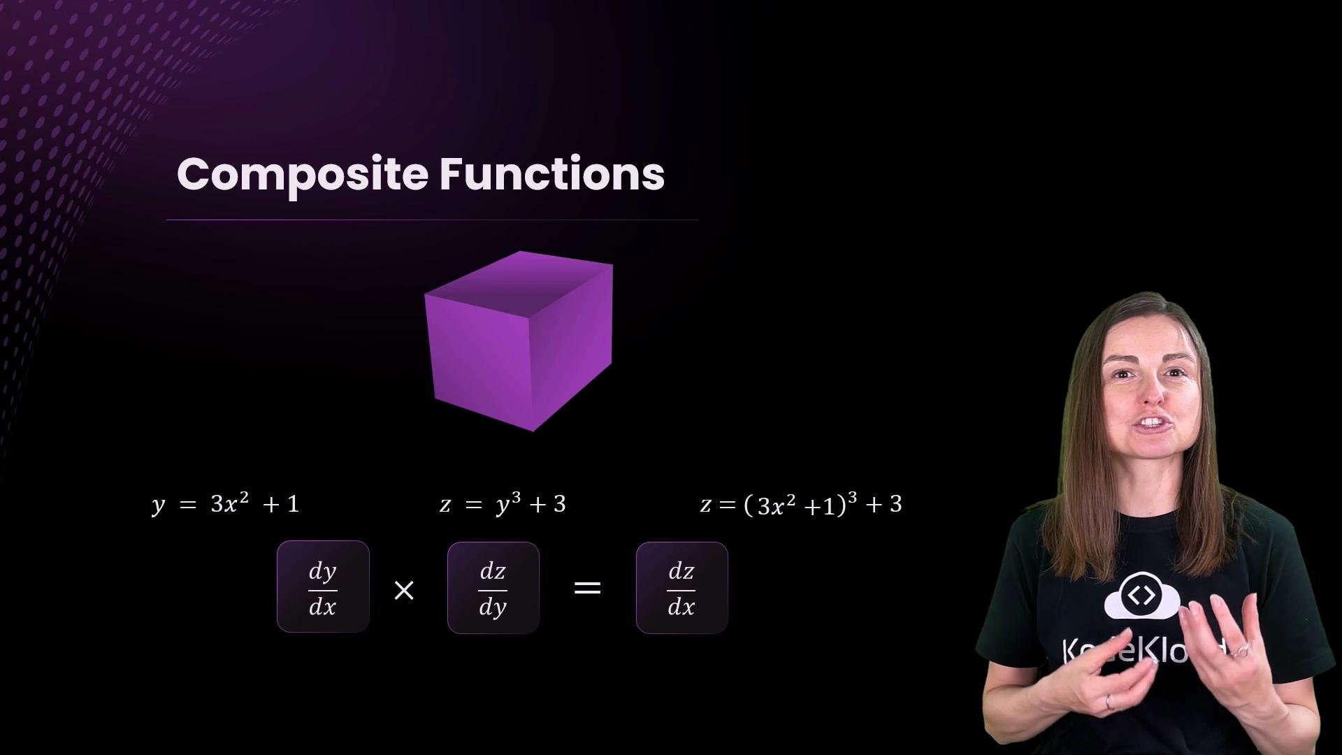
Generalization to deep networks At scale, the same pattern holds: for each weight you compute the partial derivative of the loss with respect to that weight by multiplying derivatives layer-by-layer (the chain rule). Optimizers (e.g., SGD, Adam) use these gradients to update all weights across layers. Mathematical refresh: chain rule for composite functions If y = 3x^2 + 1 and z = y^3 + 3, then z is a composite of x via y. By the chain rule:

dz/dx = (dz/dy) * (dy/dx)
dy/dx = 6x
dz/dy = 3y^2
dz/dx = 3y^2 * 6x = 18 x y^2

Replace y with (3x^2 + 1) to express dz/dx entirely in terms of x.

The image features a person presenting on the topic of composite functions, with mathematical notations for derivatives and a purple cube representing the concept visually.

Bakery analogy (another chain rule example) Let:

y = x^3 - 2
z = 2 - y^2

Then:

dy/dx = 3x^2
dz/dy = -2y
dz/dx = dz/dy * dy/dx = (-2y) * (3x^2) = -6 x^2 y

Evaluate at x = 1:

y = 1^3 - 2 = -1
dz/dx = -6 * 1^2 * (-1) = 6

This means at x = 1 a small increase in x improves z (positive derivative). The same multiplication-of-derivatives logic is exactly what backpropagation uses.

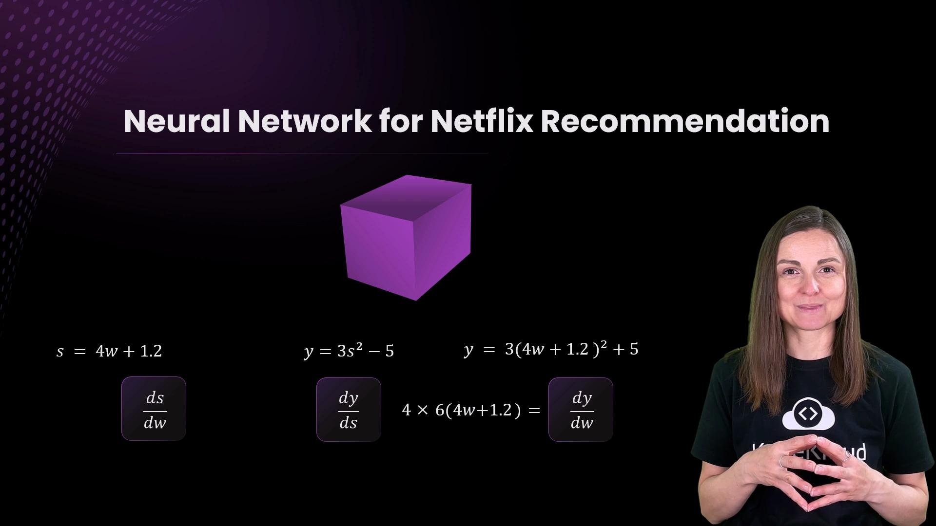
The image shows a presentation slide discussing "Neural Network for Netflix Recommendation" with mathematical equations and a speaker standing on the right.

Recap applied to the numeric network

Inner function: s = x1w1 + x2w2
Outer function: y = sigmoid(s)
Chain rule: dy/dw = (dy/ds) * (ds/dw)
The sign and magnitude of dL/dw determine whether to increase or decrease each weight.

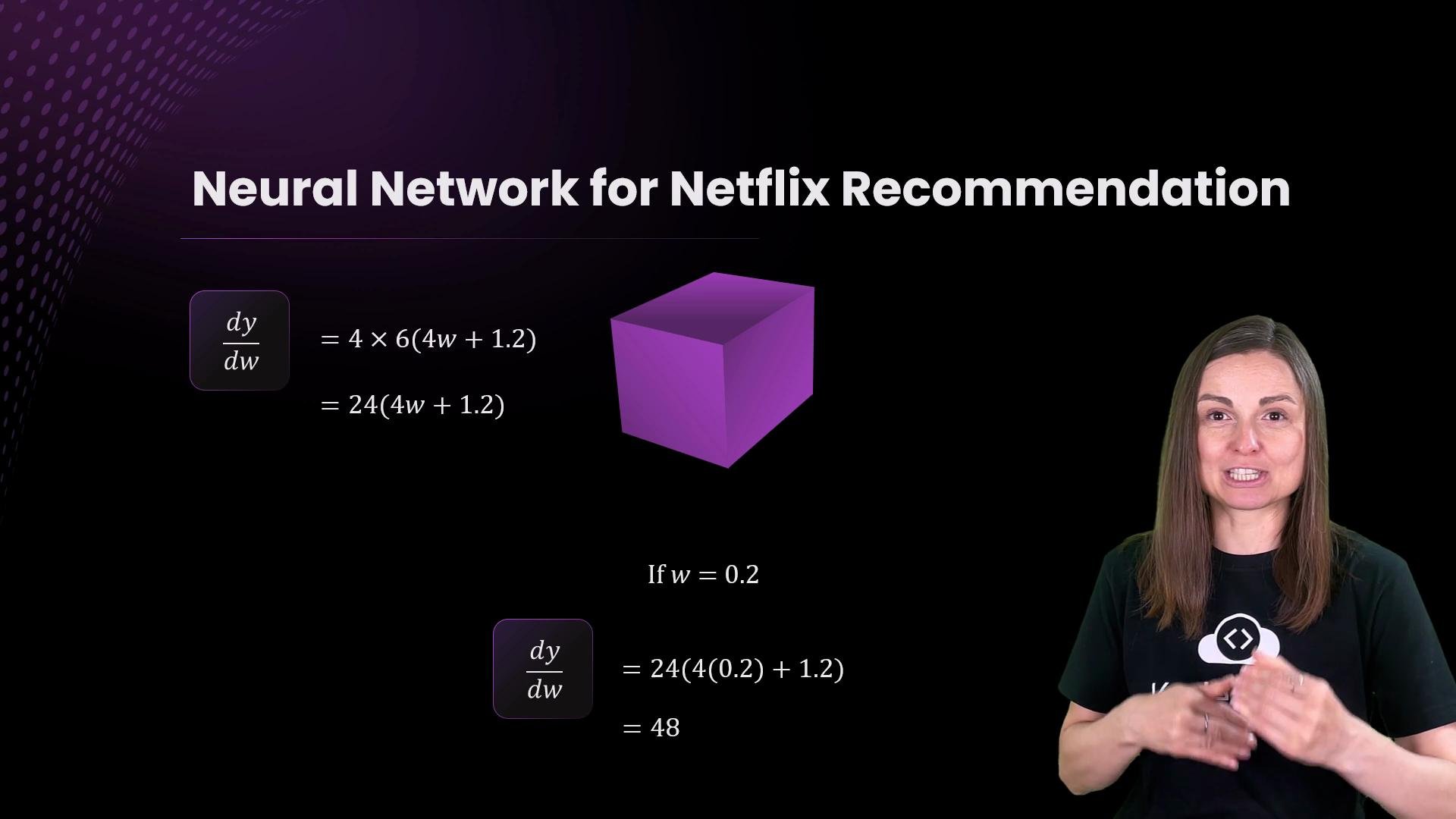
The image features text explaining a neural network for Netflix recommendations, with equations and a 3D purple cube in the background and a person speaking in the foreground.

Summary

Backpropagation = chain rule applied through network layers to compute gradients.
Gradients show how each weight affects the loss; optimizers use them to update weights and reduce error.
Repeating forward passes and backpropagation over many examples and epochs is how networks learn complex patterns.

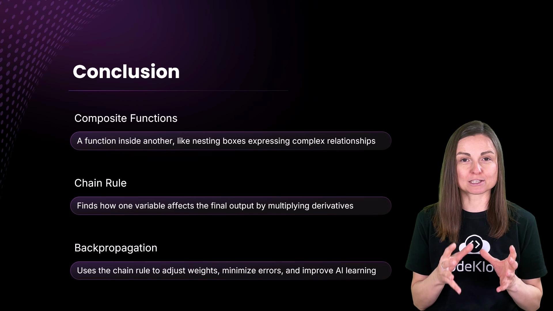
The image features a woman standing beside a presentation slide titled "Conclusion," which summarizes concepts such as composite functions, chain rule, and backpropagation.

Watch Video