Matrix Operations Part 1

Welcome — it’s Justin from KodeKloud. In this lesson we explore how matrices help computer models clean and organize sensor data for autonomous vehicles. You’ll learn how self-driving cars use matrix math to map the road, detect and avoid obstacles, and make navigation decisions. Simple matrix examples illustrate how motion and sensor transformations are handled in practice. Imagine you’re in a car with no human driver. The vehicle continuously scans the environment and collects millions of data points per second using cameras, radar, ultrasonic sensors, and LiDAR. Each sensor produces measurements from a different position and orientation on the vehicle.

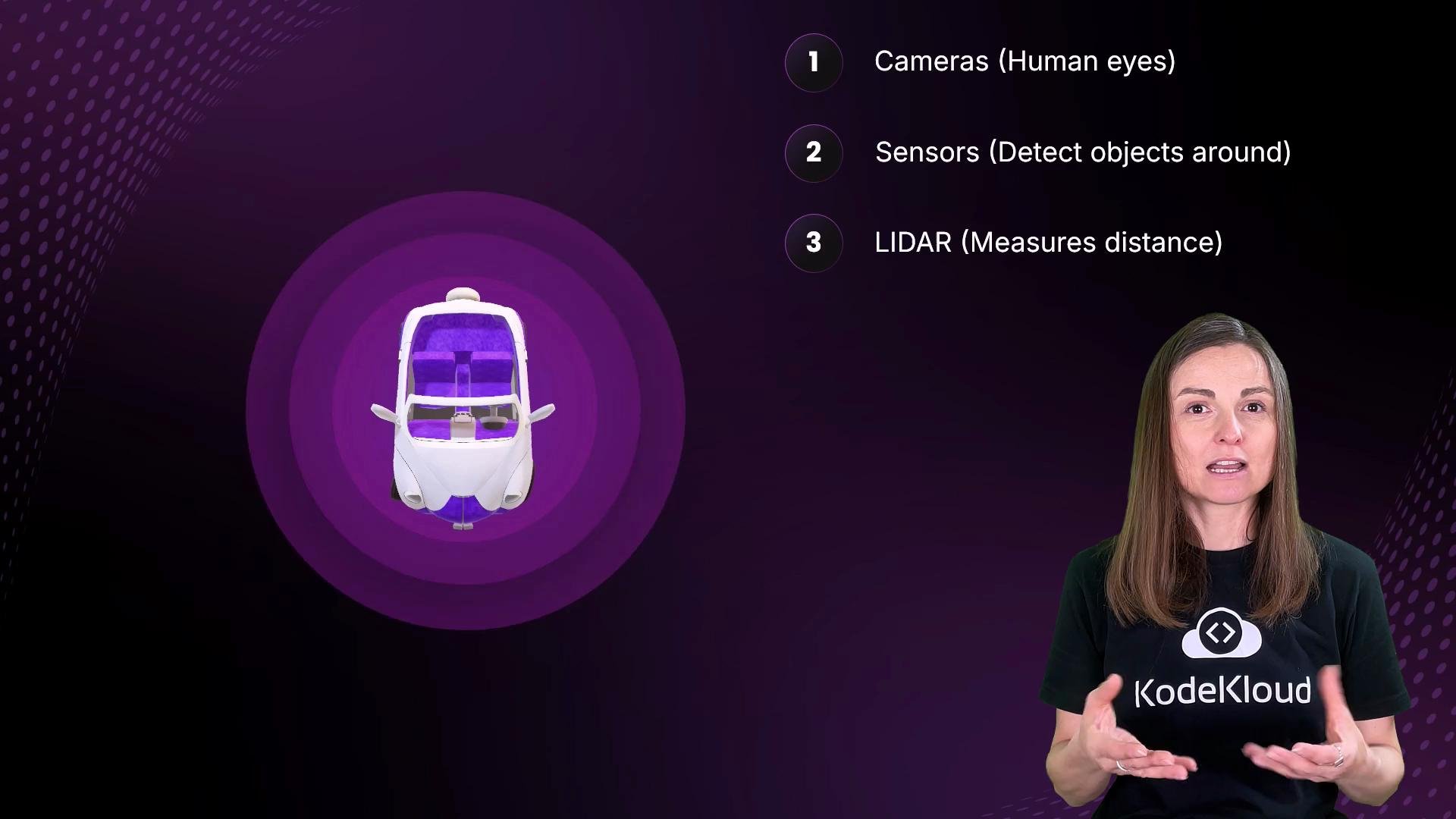
The image features a woman in a KodeKloud shirt discussing autonomous vehicle technology, with emphasis on cameras, sensors, and LIDAR for navigation. There's also a graphic of a car illustrating these technologies.

Collecting raw sensor data is only the first step. The core task is processing these measurements so the car can answer questions such as: Where are the objects around me? How far away are they? Are they moving? Machine learning models, data pipelines, and especially linear algebra (matrices) perform this work. Teams involved include machine learning engineers (perception and decision models), data scientists (safety and performance improvements), and simulation engineers (virtual testing). All of these roles rely on matrices to transform and combine sensor measurements into a coherent world model. Sensor fusion example

Different sensors can report different apparent positions for the same object because each sensor is mounted at a different place and orientation. For instance, a left-side sensor might report a pedestrian appearing to the right, while a right-side sensor reports the pedestrian to the left — the pedestrian is actually ahead.
The vehicle knows each sensor’s pose (position and orientation). Using transformation matrices, the vehicle converts each sensor’s measurements into a common coordinate frame (the vehicle frame) and then combines them into a unified map.

Here’s an illustrative sensor snapshot: LiDAR detects three objects — a tree, a traffic light, and a pedestrian. We can store these detections in a matrix where each row is an object and each column is a property (distance, height, moving flag). To fuse data across sensors, convert each sensor’s matrix into the vehicle frame by left-multiplying it (or otherwise applying) that sensor’s transformation matrix, then aggregate the transformed rows. Matrix multiplication is the core operation enabling these transformations. Let’s review how matrix multiplication works and the rules that govern it. Multiplying square matrices Square matrices have the same number of rows and columns — for example 2×2 or 3×3. Two square matrices of the same size can be multiplied together. Matrix multiplication is based on dot products:

To compute one element of the product matrix, take a row from the first matrix and a column from the second matrix, multiply corresponding elements pairwise, and sum the results.
Example scalar calculation: multiply 5 × 3 and 2 × 2 then sum to get 15 + 4 = 19. That sum is one element of the resulting matrix.

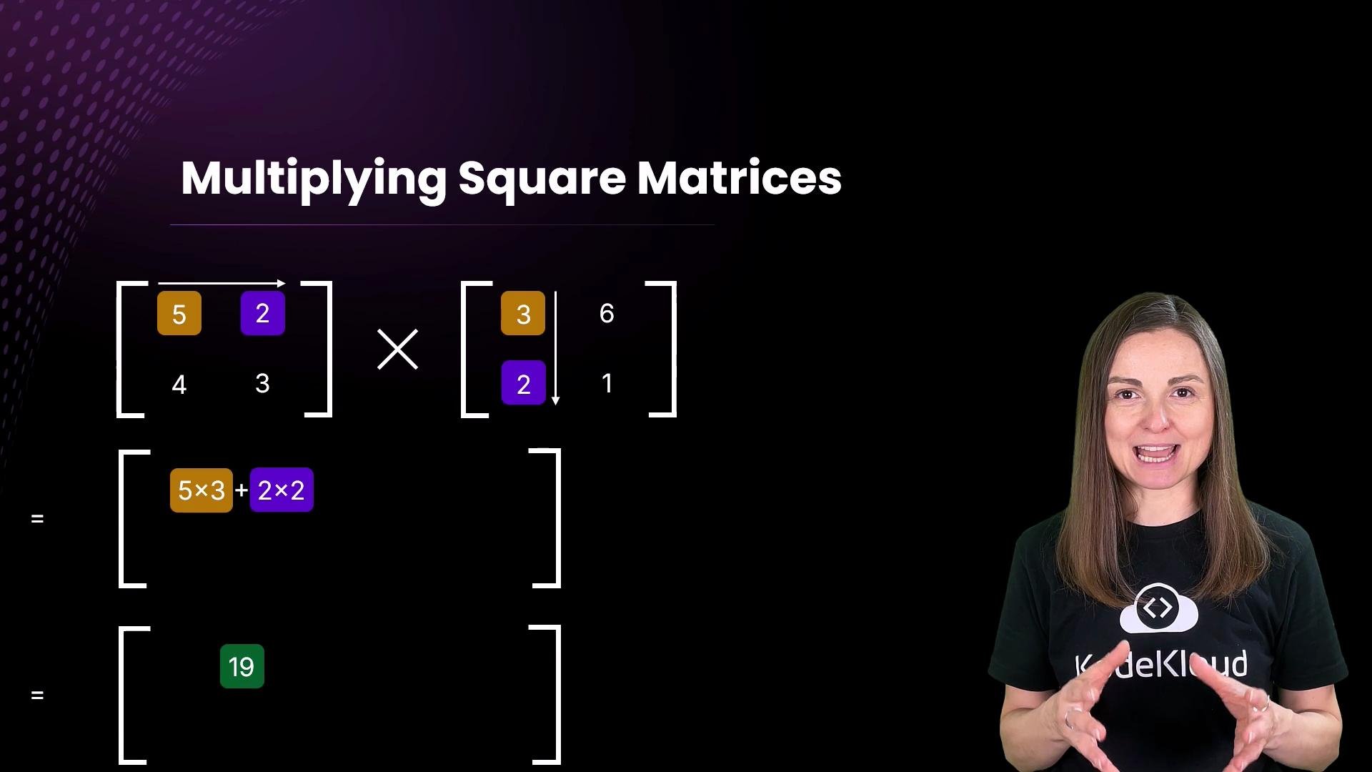
The image illustrates the process of multiplying square matrices, showing the calculation of an element in the resulting matrix, alongside a person explaining the concept.

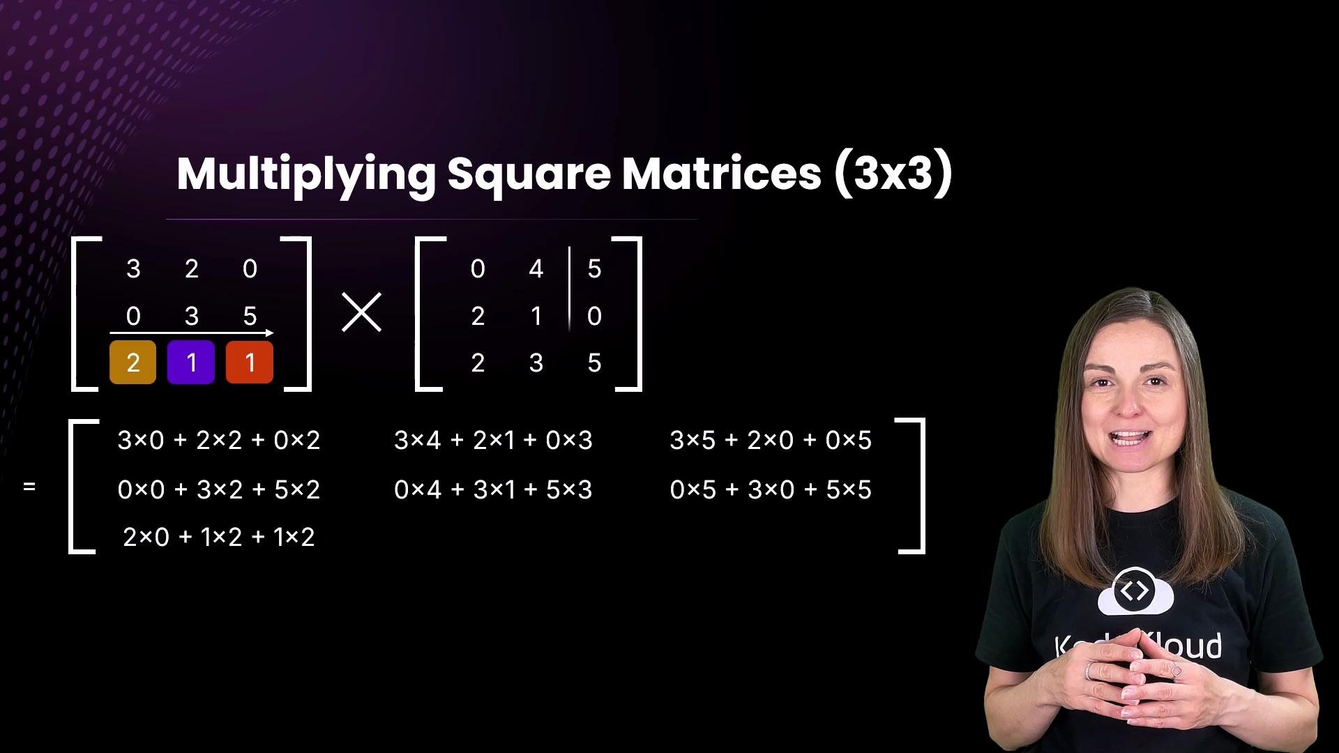
Repeat that dot-product process for every row of the first matrix and every column of the second matrix to fill the result. For a 3×3 example, you compute:

First row of A with first column of B (dot product)
First row of A with second column of B
First row of A with third column of B
Then repeat for the second and third rows of A

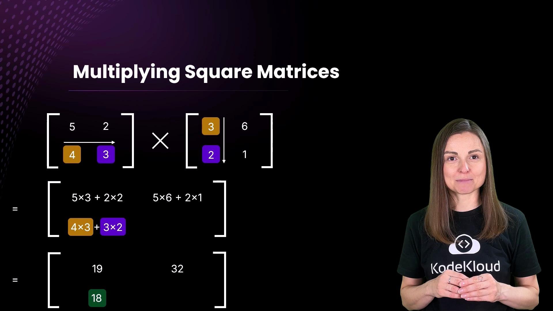
The image illustrates the process of multiplying square matrices, showing two matrices being multiplied and detailing the calculations involved. A person is also visible on the right side of the image, wearing a shirt with text.

The same step-by-step dot-product approach applies to any 3×3 multiplication as well.

The image illustrates the process of multiplying two 3x3 matrices, showing the mathematical steps involved. It also features a person standing on the right side.

General matrix multiplication rule

If A is an m × n matrix and B is an n × p matrix, then the product A × B is defined and has shape m × p.
In plain terms: the number of columns of the first matrix must equal the number of rows of the second matrix.

Matrix multiplication is only possible when the first matrix’s column count matches the second matrix’s row count. The resulting matrix has the number of rows of the first matrix and the number of columns of the second matrix.

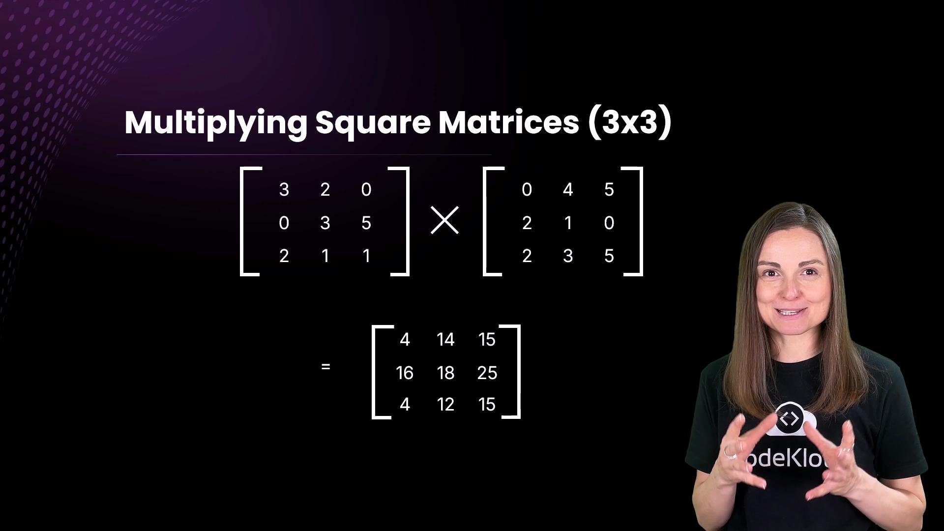
The image shows the multiplication of two 3x3 matrices with the resulting matrix, alongside a person explaining the process.

Common size examples

First matrix (A)	Second matrix (B)	Multiplication possible?	Result shape
`2×2`	`3×2`	No — `2` columns ≠ `3` rows	N/A
`2×3`	`3×2`	Yes	`2×2`
`3×3`	`3×3`	Yes	`3×3`
`3×2`	`2×4`	Yes	`3×4`

Notes on multiplication validity

If A has 3 columns and B has 2 rows, multiplication A×B is not defined because the inner dimensions don’t match.
If A has 3 columns and B has 3 rows, A×B is defined.

A common pitfall: matrix multiplication is not commutative. If A × B is defined, B × A might be undefined or yield a different-shaped/result matrix. Always check shapes before multiplying.

Applying this to sensor fusion

Each sensor produces a detection matrix (rows = objects, columns = properties).
Each sensor has a corresponding transformation matrix that maps sensor coordinates into the vehicle coordinate frame.
Convert a sensor’s detections into the vehicle frame by multiplying with its transformation matrix (shape must align).
After transforming each sensor’s rows into the vehicle frame, concatenate or otherwise aggregate the rows to form the vehicle’s perception matrix.
This combined, transformed matrix becomes the input to higher-level algorithms such as tracking, object classification, and path planning.

Watch Video