

1. Simple example: f(x, y) = x^2 + y^2
When computing a partial derivative, treat all other variables as constants.- ∂f/∂x: treat y as constant → derivative of x^2 is 2x, derivative of y^2 is 0. So
∂f/∂x = 2x. - ∂f/∂y: treat x as constant → derivative of y^2 is 2y, derivative of x^2 is 0. So
∂f/∂y = 2y.

-∇f.
2. A slightly more complex function: f(x, y) = x^3 + y^3 + xy
Next example introduces higher powers and an interaction term.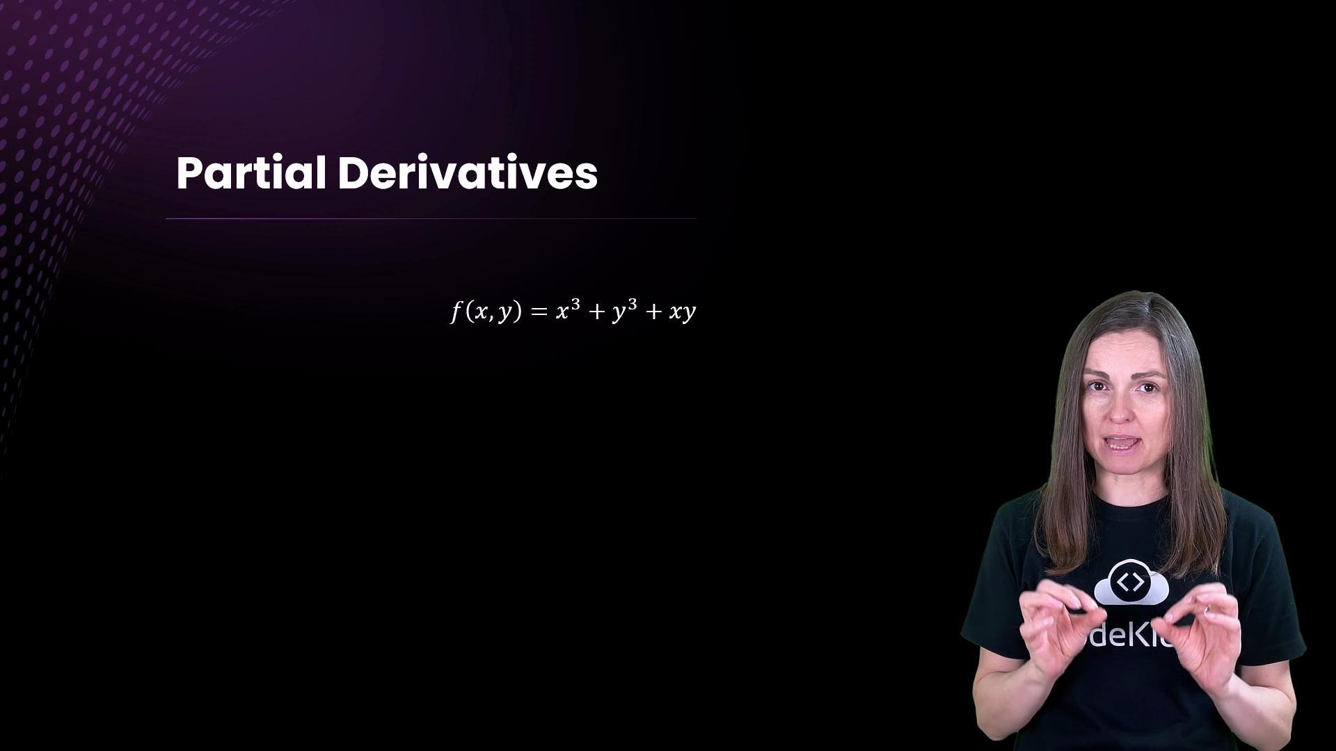
-
∂f/∂x: derivative of
x^3is3x^2;y^3is constant → 0; derivative ofxyw.r.t. x isy.
So∂f/∂x = 3x^2 + y. -
∂f/∂y: derivative of
y^3is3y^2;x^3is constant → 0; derivative ofxyw.r.t. y isx.
So∂f/∂y = 3y^2 + x.
[4, 4] indicates the steepest increase direction at (1,1). To reduce the function value, move opposite this vector.
3. Travel-time model: Susie’s delivery route
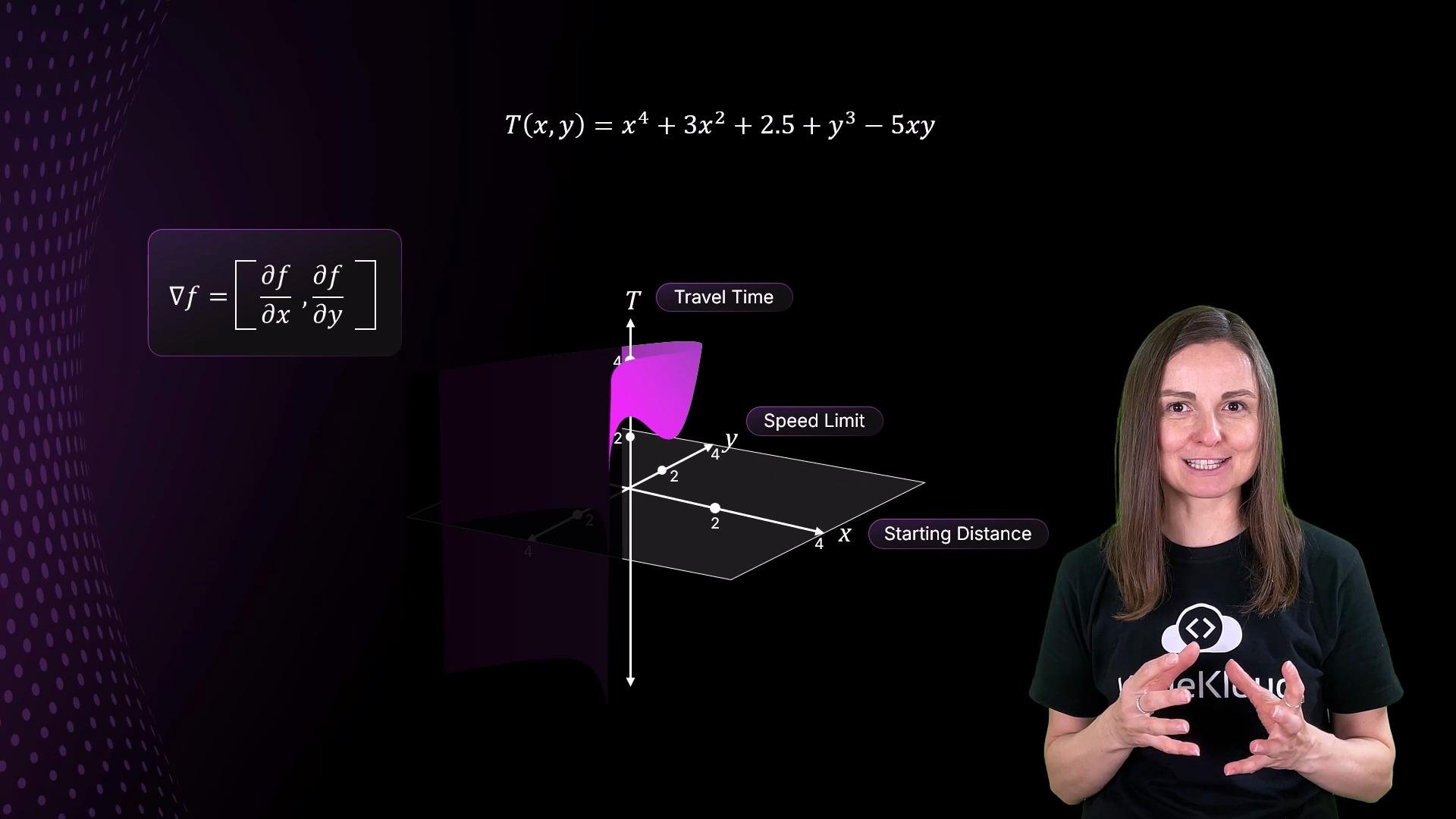
We now apply partial derivatives to a travel-time model. Let T(x, y) be Susie’s travel time depending on distancex and speed-limit-related variable y.
Example model:
T(x,y) = x^4 + 3x^2 + 2.5 + y^3 - 5xy
-
∂T/∂x:
- d/dx(
x^4) =4x^3 - d/dx(
3x^2) =6x - d/dx(
2.5) =0 - d/dx(
y^3) =0(y constant) - d/dx(
-5xy) =-5y=>∂T/∂x = 4x^3 + 6x - 5y
- d/dx(
-
∂T/∂y:
- d/dy(
y^3) =3y^2 - d/dy(
-5xy) =-5xAll other terms are constant in y =>∂T/∂y = 3y^2 - 5x
- d/dy(
[5, -2] points to the direction that increases travel time most rapidly. A positive first component means increasing x (distance) tends to increase time; a negative second component means increasing y (speed-limit variable) tends to reduce time. Thus, to reduce travel time, move opposite the gradient.
Gradient descent update (one step):
new_position = current_position - learning_rate * gradient. Recompute partial derivatives at the new position and repeat until convergence.4. Real-time routing example (Susie on a scooter)
Susie trusts the app’s computed route. If traffic changes, the app updates variables and recomputes the gradient to adapt the route.
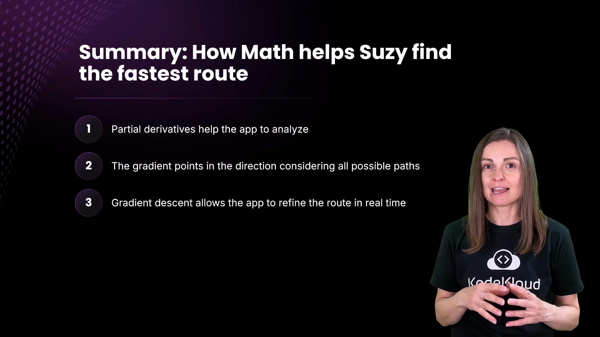
- Model travel time as a multivariable function (distance, speed, traffic, signals).
- Compute partial derivatives to measure local sensitivity of time to each variable.
- Combine partials into the gradient: the direction of greatest increase.
- Use gradient descent: iteratively step in the negative-gradient direction to decrease travel time.
5. Where this math is used
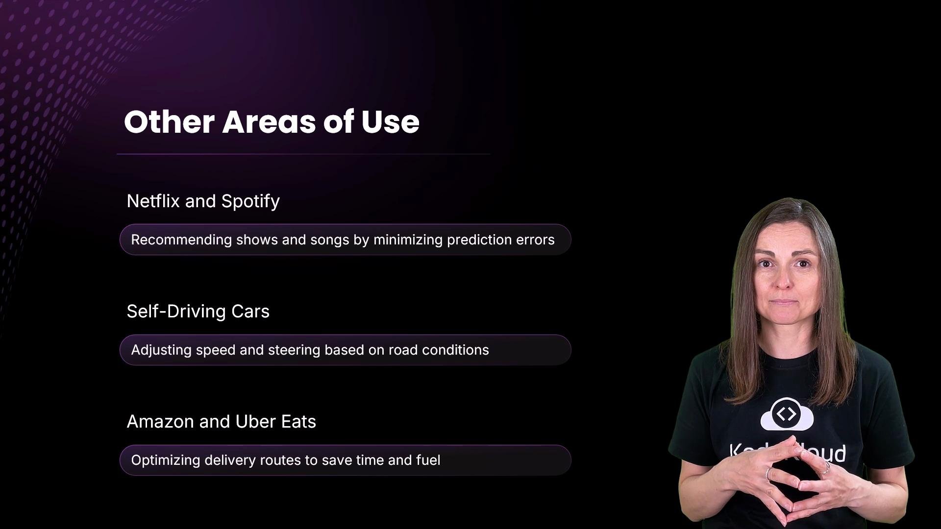
Gradient-based optimization is foundational in many modern systems:- Recommendation engines (Netflix, Spotify) — minimize prediction error.
- Self-driving vehicles — continuous control optimization with sensor inputs.
- Logistics (Amazon, Uber Eats) — routing and fuel/time minimization.
- Machine learning — neural network training via variants of gradient descent.
Quick reference: common derivative rules
Final takeaway
- Partial derivatives quantify how each independent variable affects the output locally.
- The gradient bundles partials into the direction of steepest ascent.
- Gradient descent follows the negative gradient to find minima, making it a powerful tool for optimization in routing, ML, control systems, and more.