

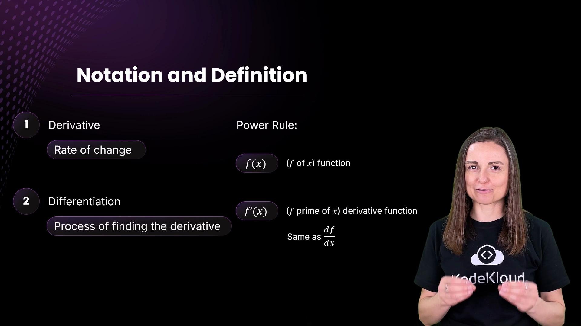
f(x) denotes a function, then f'(x) denotes its derivative — the instantaneous rate of change of f at x. Understanding derivatives is essential for physics, engineering, machine learning, and computer vision.
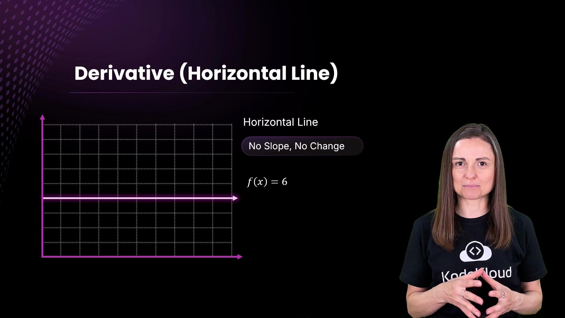
f(x) = 6 — its value does not change as x changes. The derivative measures change, so the derivative of a constant is zero:
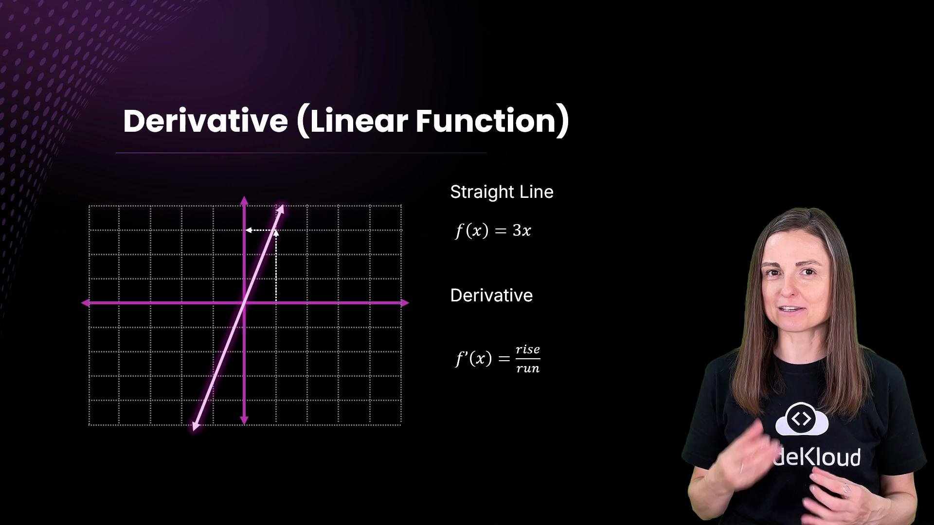
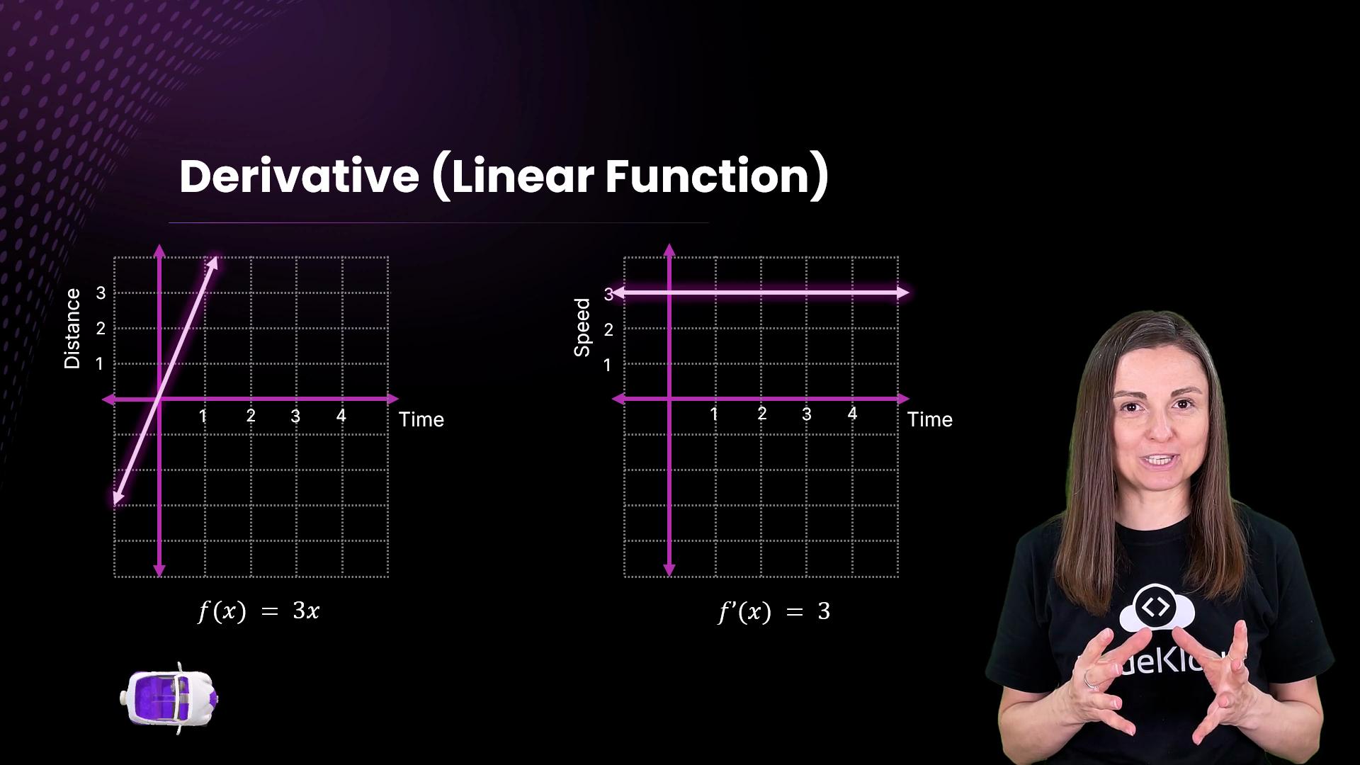
f(x) = 3x has slope 3: if the rise is 3 and the run is 1, the slope is 3. If f(x) models distance over time, the speed is constant.
x. To find the slope at a specific point we draw the tangent line — the straight line that just touches the curve at that point — and measure its slope there.
Consider the quadratic f(x) = x^2. The slope (derivative) differs at various x values:
- At
x = −1, the tangent slopes downward:f'(−1) = −2. - At
x = 0, the tangent is horizontal:f'(0) = 0. - At
x = 1, the tangent slopes upward:f'(1) = 2.
x yields f'(x) = 2x — the derivative of x^2.
When f(x) represents distance and f'(x) represents velocity, the steepness of the distance graph corresponds to speed: steep = fast, flat = slow, zero slope = stopped. A sign change in the derivative indicates a change in direction.
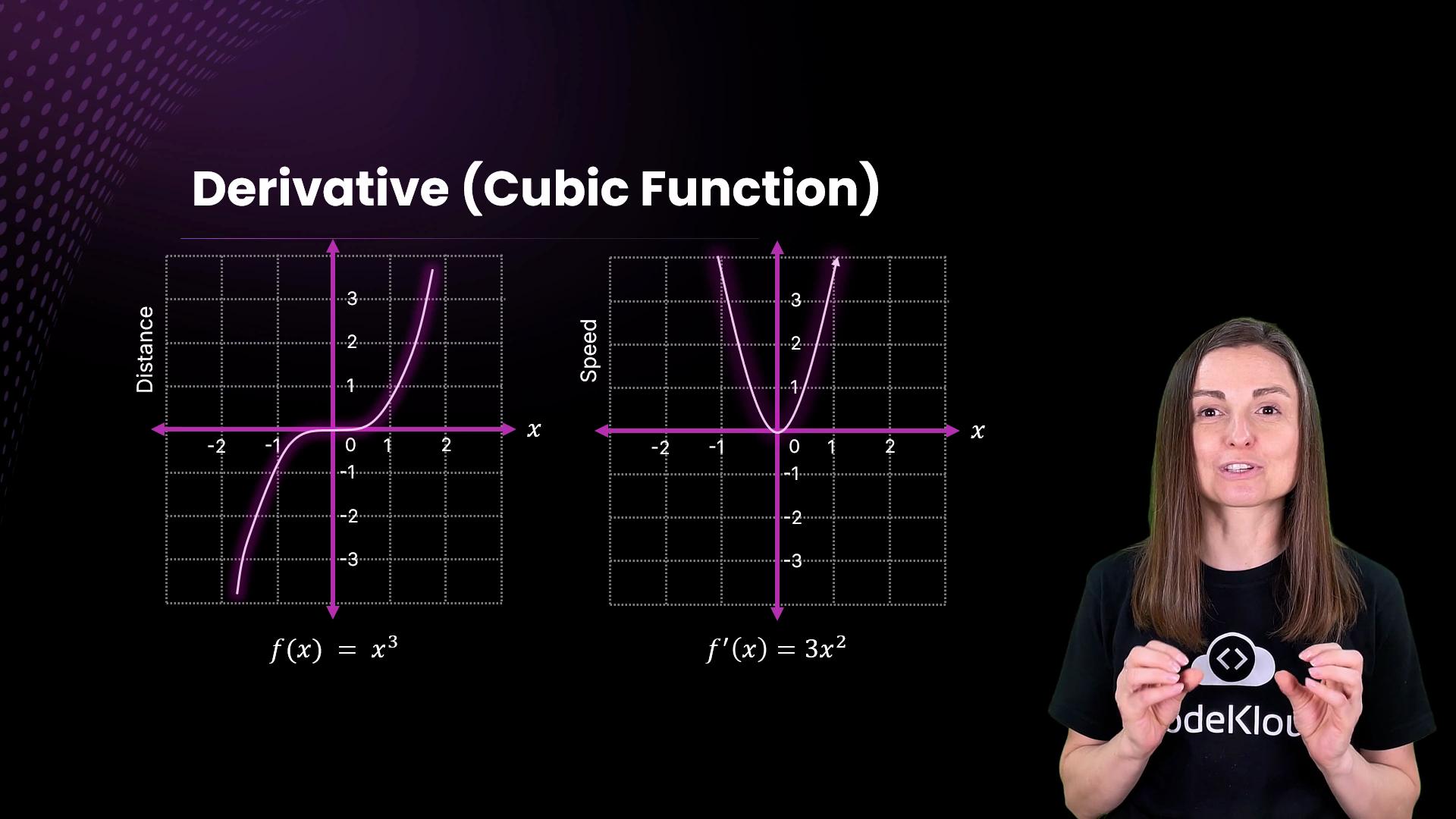
For higher powers the pattern continues. Example: for f(x) = x^3, the derivative is f'(x) = 3x^2. The distance and derivative graphs together capture slowing, stopping, and speeding up.
f(x) = x^4 and you get f'(x) = 4x^3.
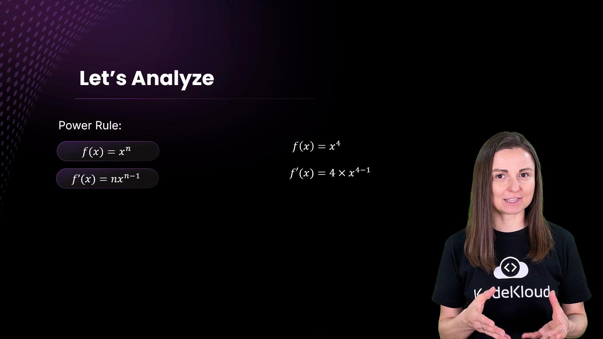
-
Constant multiple rule: if a constant
amultiplies the power, multiply the coefficient by the power.Example:f(x) = 5x^3→f'(x) = 15x^2. -
Linearity (sum rule): differentiate each term separately.
Example:
Back to the car example
Suppose the distance-to-roadworks as a function of time is:
f'(x) gives the instantaneous rate of change of distance with respect to time. For instance:
f'(0) = -80 means the distance is decreasing at 80 units per time unit at x = 0. The derivative is a signed rate (negative indicates motion toward the roadworks). Speed, as commonly used, is the non-negative magnitude of velocity.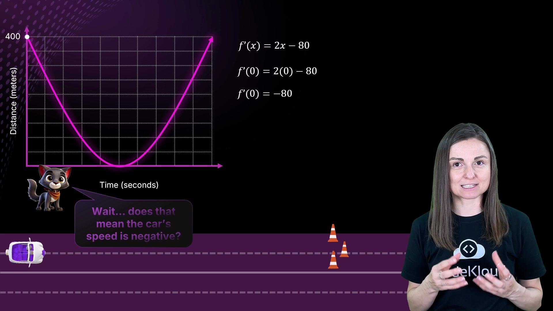
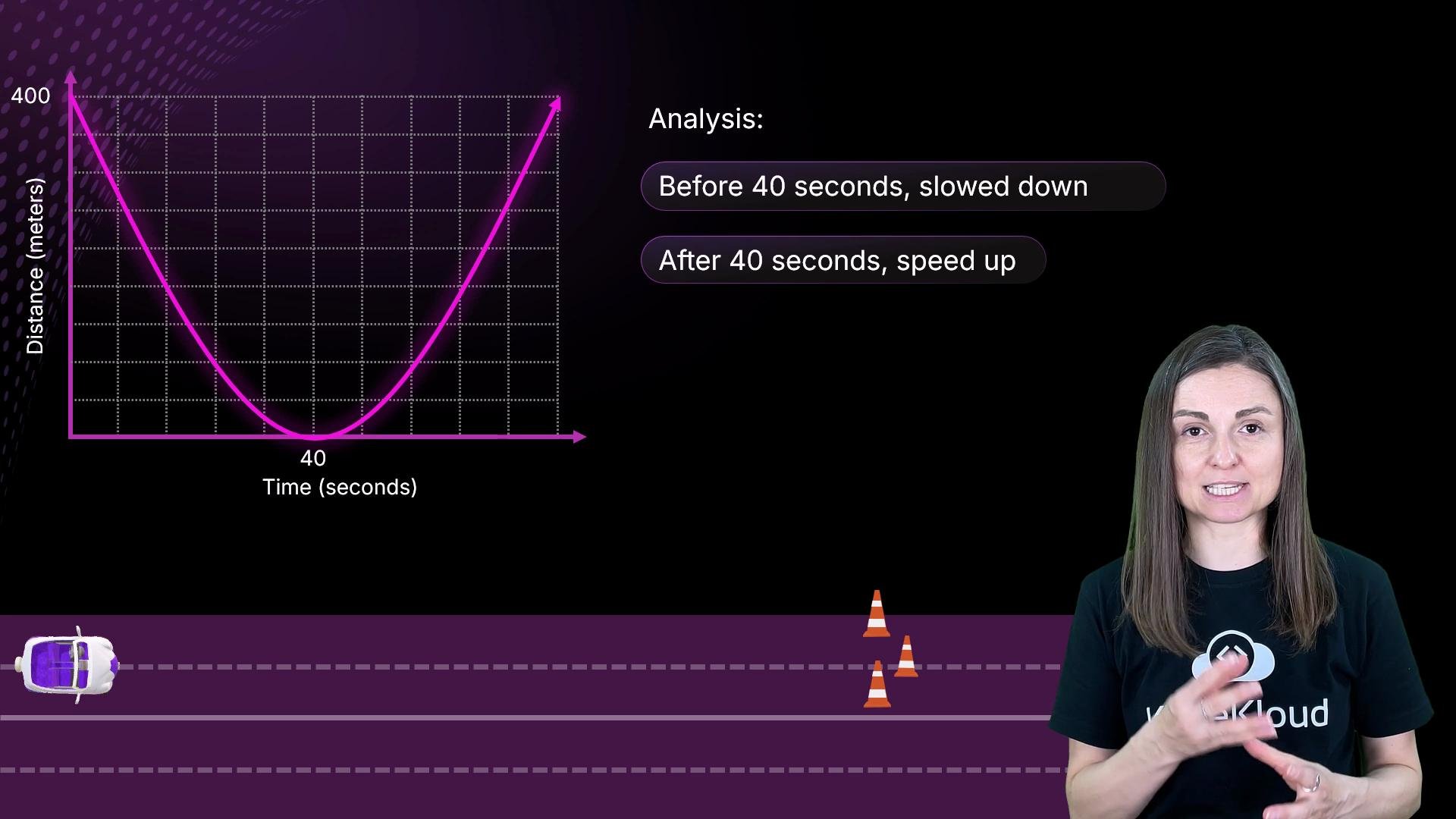
f'(x) = 0:
f'(40) = 0. At x = 40 seconds the distance is neither increasing nor decreasing — the car is at its closest point to the roadworks. Before x = 40 the distance is decreasing (f'(x) < 0); after x = 40 it is increasing (f'(x) > 0).
-
Self-driving cars
- compute instantaneous speed and direction (is distance increasing or decreasing),
- decide braking or acceleration,
- smooth acceleration/braking for comfort,
- predict trajectories for safe lane changes and collision avoidance.
-
Computer vision and machine learning
- an image is a grid of pixel intensities (e.g.,
0to255), - computing differences between neighboring pixels approximates discrete derivatives,
- these discrete derivatives highlight edges and motion (sharp local changes appear as peaks),
- repeated derivatives across rows/columns help detect shapes and moving objects.
- an image is a grid of pixel intensities (e.g.,
- A derivative measures how fast a quantity changes at a point.
- The power rule (
f(x) = x^n→f'(x) = n x^(n-1)) makes differentiating polynomials quick and systematic. - Interpreting derivatives connects math to real-world systems (self-driving cars) and machine perception (edge detection).
- Khan Academy — Derivatives Intuition
- MIT OpenCourseWare — Single Variable Calculus
- Stanford — Computer Vision: Edge Detection Concepts