Welcome — it’s Justyna from KodeKloud. In this lesson we introduce probability: the mathematics of uncertainty. Probability is not guesswork or certainty — it quantifies how likely events are. We use it across domains: weather forecasting, medical decision-making, traffic modeling, and machine learning. This article explains how probability distributions help make uncertain outcomes (like rain) actionable. We’ll cover simple yes/no events (Bernoulli), repeated yes/no experiments (Binomial, briefly referenced), and the Normal distribution (overview) with a focus on how these ideas improve weather predictions.
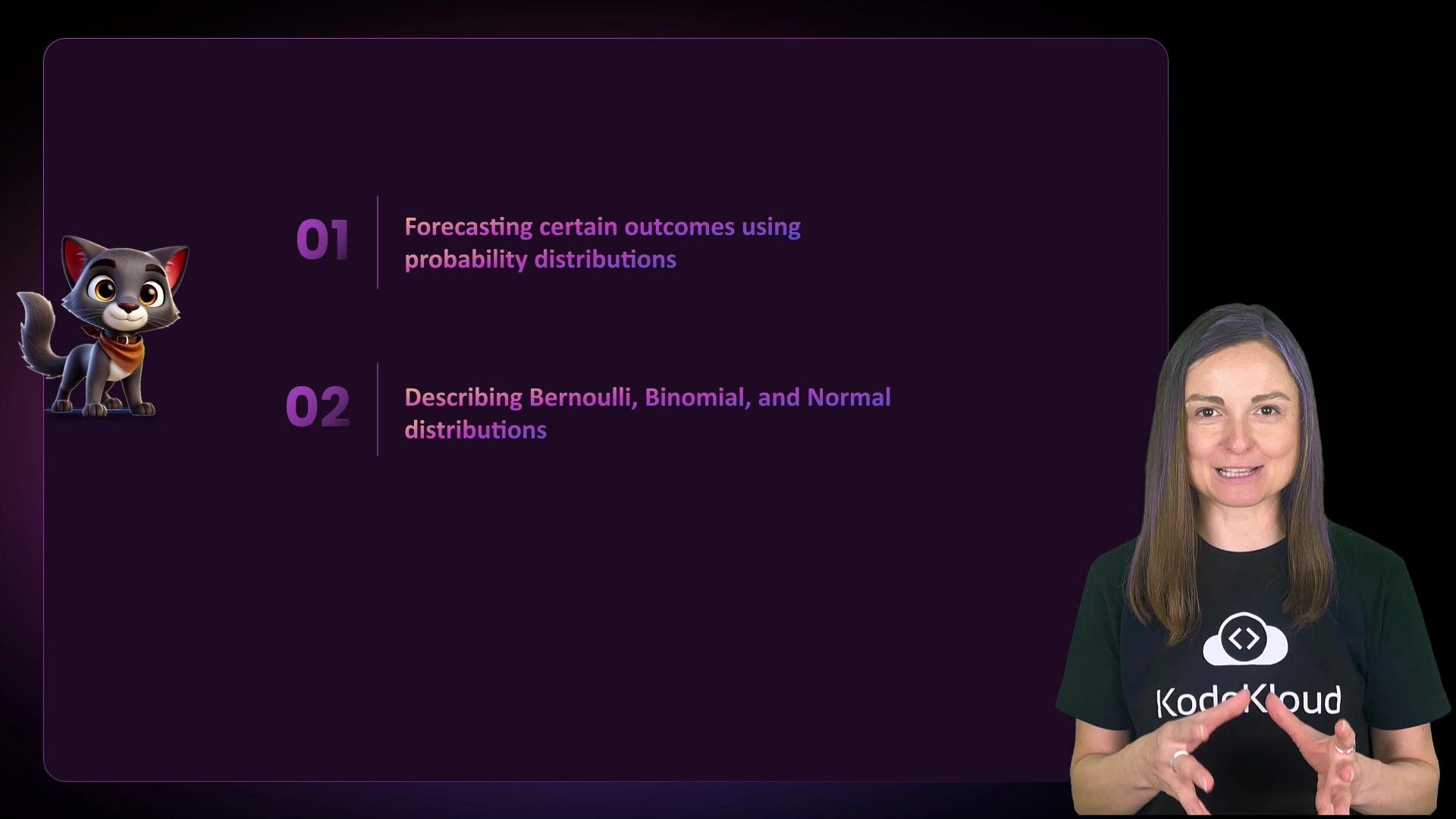
The image shows a presentation slide with two points about probability distributions, alongside an animated character on the left and a person on the right.
Why does a forecast say “70% chance of rain”? That phrasing causes confusion: does it mean 70% of the time, 70% of the area, or something else? Below we clarify the typical interpretation and show how distributions formalize that uncertainty. Data scientists, machine learning engineers, and meteorological analysts each use probability differently:
  • Data Scientists analyze historical weather to estimate patterns and probabilities.
  • Machine Learning Engineers train models that output probability estimates.
  • Meteorologists integrate models, observations, and expertise to produce forecast probabilities.

The image shows a weather app indicating a 70% chance of rain in Tampa, FL, alongside the question "Why does a 70% chance of rain confuse us?" and a person gesturing with their hands.
The image depicts a presentation slide titled "Job Relevance" featuring illustrations of three roles: Data Scientist (Weather Tech), Machine Learning Engineer, and Meteorological Data Analyst. A person is also present beside the illustrations, gesturing as if explaining.
Meet Jane. It’s Thursday evening and she checks the weather app to decide what to wear and whether to bring an umbrella. The app shows a 70% chance of rain at 6–7 p.m.
The image features an illustration of a person with an umbrella checking a weather app, and a person speaking next to the app's display. The app shows rain probability and weather conditions throughout the day.
Interpretation: the forecast means there is a 70% chance that rain will occur somewhere in the forecast area at some point during that hour. It does not specify how long it will rain or exactly where within the area it will rain. Forecast probabilities are statements about likelihoods, not precise timings or durations.
The image shows a woman standing next to a weather forecast display with a 70% chance of rain, alongside an illustration of a person holding an umbrella in the rain.
Forecasts come from models and observations combined with probability theory. To formalize that process we use random variables and probability distributions.

Random variables: discrete vs continuous

A random variable maps outcomes to numbers so we can analyze uncertainty mathematically.
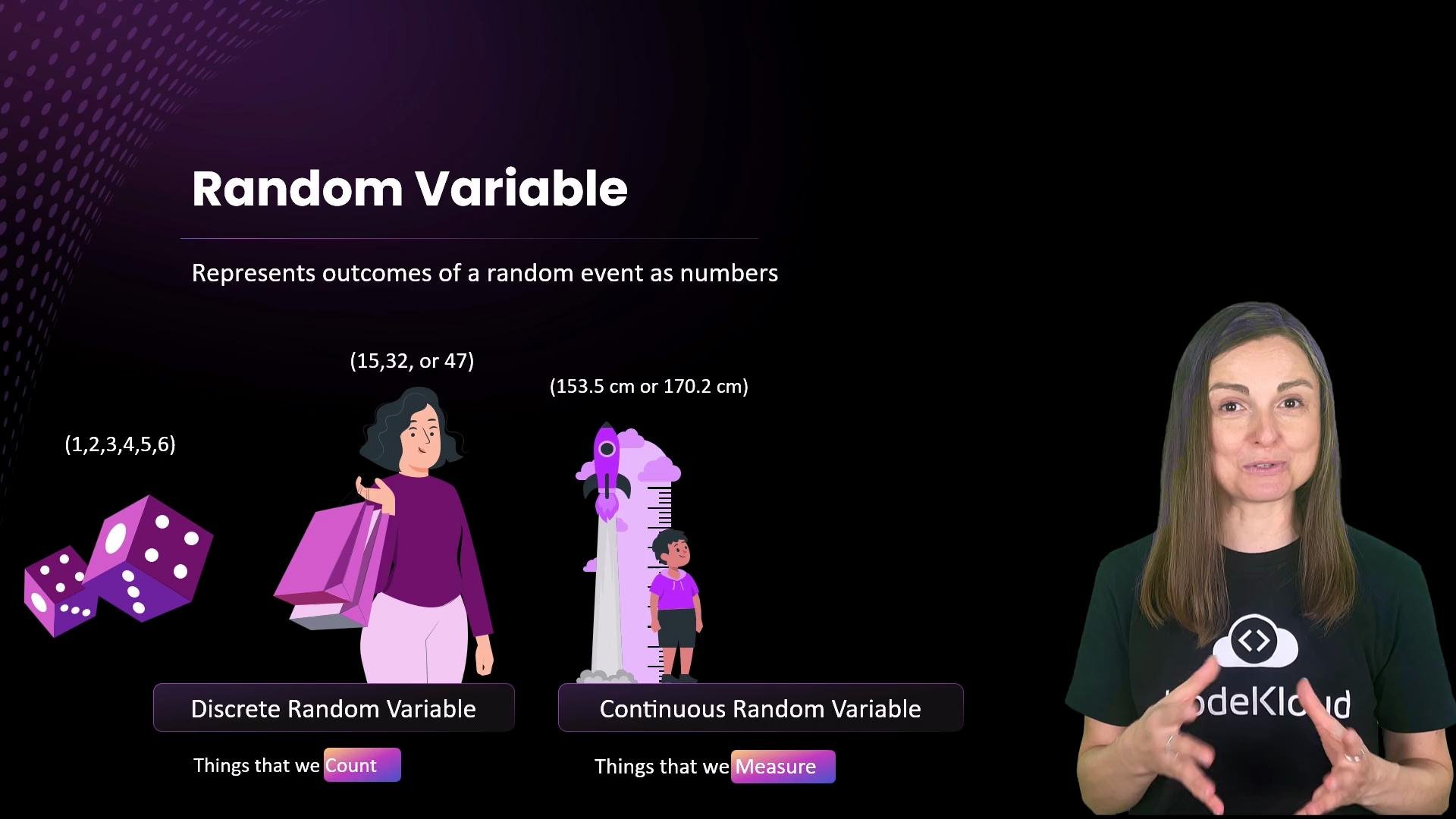
TypeWhat it representsExamples
DiscreteCountable outcomesdie roll = {1,2,3,4,5,6}, number of customers = 15
ContinuousMeasured values on a continuumheight = 170.2 cm, temperature = 21.7 °C
The image explains the concept of random variables with illustrations of discrete (things that we count) and continuous random variables (things that we measure), featuring a person and a graphical representation.
Non-numeric outcomes (like “rain” vs “no rain”) can be encoded numerically so probability models apply. For example: rain = 1, no rain = 0. These encoded values let us treat categorical events as random variables. A probability distribution assigns probabilities to each possible outcome. For a fair six-sided die:
P(1) = 1/6, P(2) = 1/6, ..., P(6) = 1/6, which we can visualize as a bar chart.
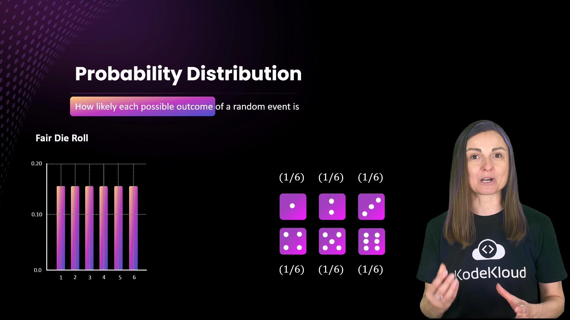
The image demonstrates a probability distribution of a fair die roll, showing equal likelihood for each outcome with a chart and dice illustrations. A person is presenting the concept, wearing a KodeKloud shirt.
Next, we focus on distributions especially relevant to forecasting: Bernoulli (single yes/no), Binomial (repeated trials), and the Normal distribution (continuous clustering around a mean).

Bernoulli distribution — single yes/no events

The Bernoulli distribution models a single trial with two outcomes: success (1) or failure (0). Typical use cases include “raining vs not raining”, “spam vs not spam”, or “positive vs negative test”. For a Bernoulli random variable X with success probability p, the probability mass function (PMF) can be written compactly:
P(X = x) = p^x * (1 - p)^(1 - x)   for x in {0, 1}
This expression gives the two probabilities explicitly:
  • P(X = 1) = p
  • P(X = 0) = 1 − p
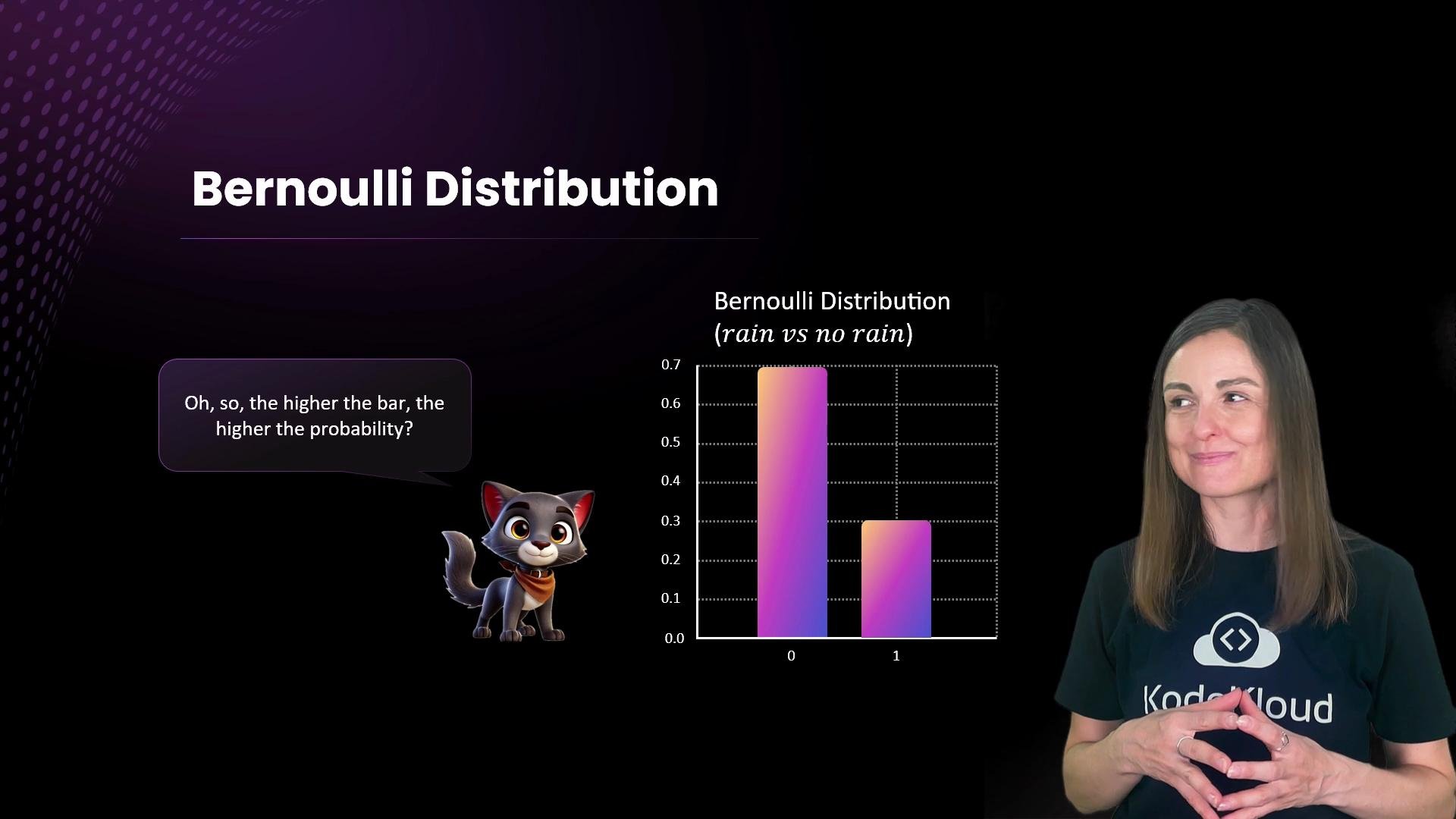
Example: if p = 0.7 for rain:
P(X = 1) = 0.7     (rain occurs)
P(X = 0) = 0.3     (no rain)
The image illustrates a Bernoulli distribution with a graph comparing the probability of rain vs no rain and includes a cartoon character discussing probability with a person standing next to the graph.
A fair coin flip is a Bernoulli trial with p = 0.5. If both bars are 50% each, outcomes are equally likely.
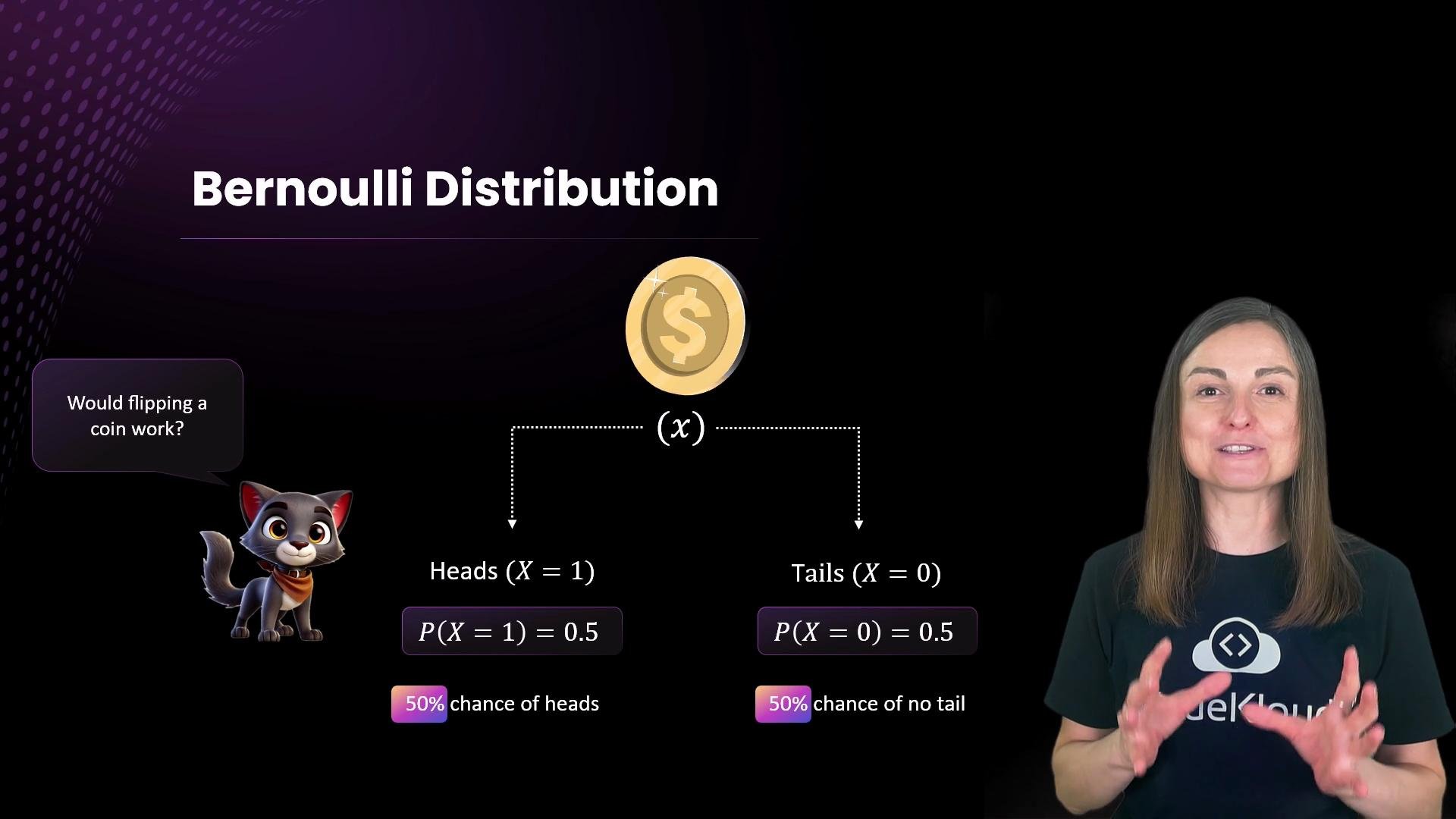
The image explains the Bernoulli Distribution using a coin flip example, illustrating equal probabilities for heads and tails, alongside a cartoon character asking a question.
Why use the compact PMF formula? Because it:
  • Encodes both outcomes in one expression,
  • Is trivial to implement in code and statistical libraries,
  • Serves as a building block for more complex models (e.g., Binomial, logistic regression, Bernoulli likelihoods in Bayesian inference).
Short calculation recap for p = 0.7:
P(X = 1) = p^1 * (1 - p)^0 = 0.7
P(X = 0) = p^0 * (1 - p)^1 = 0.3
The image illustrates the Bernoulli formula with a graph comparing the probability of rain vs no rain and includes a cartoon character discussing probability with a person standing next to the graph.
Where does p come from? From data and models. Meteorologists combine historical observations, model ensembles, and simulations to estimate probabilities. For example, if 7 out of 10 model ensemble members predict rain, that supports p ≈ 0.7. Probabilities summarize evidence, not guarantee single outcomes.
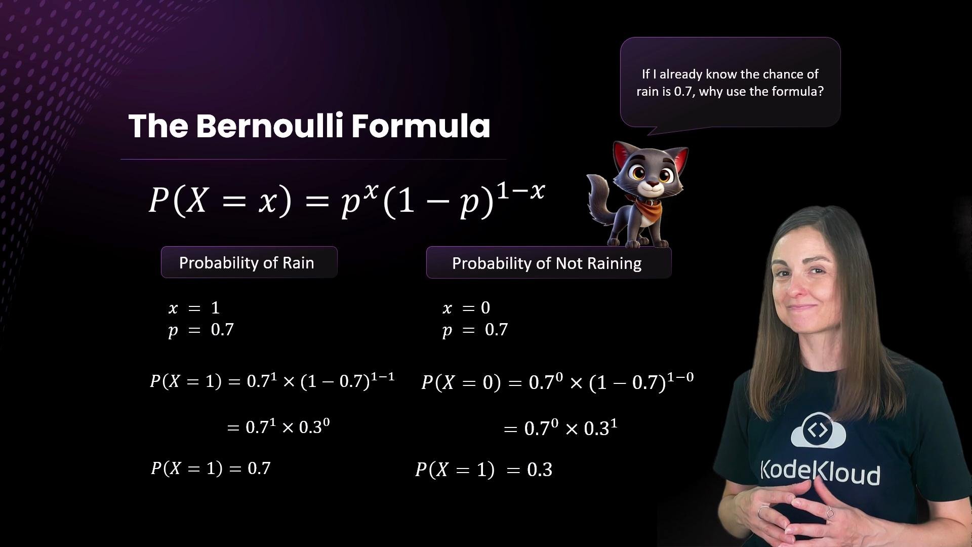
The image explains the Bernoulli formula, showing calculations for the probability of rain and not raining, with a cat character and a person alongside it.

Expected value of a Bernoulli

The expected value (mean) E[X] describes the long-run average outcome after many independent trials. For Bernoulli X:
E[X] = (1 × P(X = 1)) + (0 × P(X = 0)) = 1 × p + 0 × (1 − p) = p
So when p = 0.7, E[X] = 0.7. That is why a 70% predicted probability can be read as a long-run fraction of occurrences.
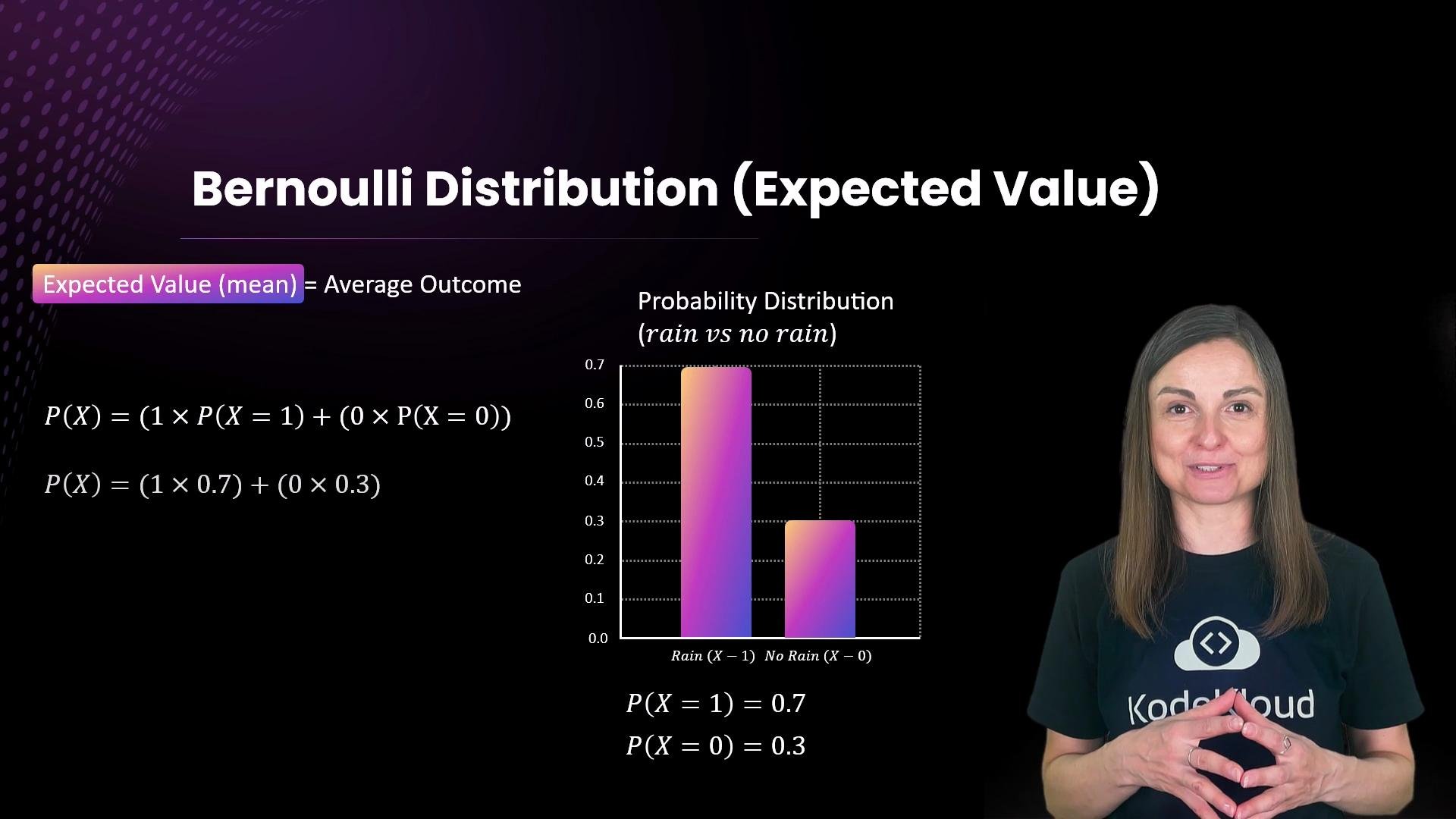
The image features a presentation slide on the Bernoulli Distribution, showing the expected value (mean) calculation with a probability distribution chart for rain vs. no rain. There's also a person standing to the side of the slide.
Bernoulli distributions are compact but powerful: they underpin binary classifiers, components of weather simulation pipelines, A/B tests, and probabilistic modeling in machine learning.
The Bernoulli distribution models single yes/no outcomes. Its expected value equals the success probability p, which is why a predicted probability (like 70%) can be interpreted as the long-run fraction of successes.

Quick references and further reading

For the next lesson we’ll build on Bernoulli trials to discuss repeated trials (Binomial distribution) and continuous-valued distributions such as the Normal distribution and how they apply to forecasting and model evaluation.

Watch Video