In this lesson we compute the inverse of a 2×2 matrix, verify the result by multiplication, and explain why the determinant determines invertibility. Understanding 2×2 inversion is a foundation for solving linear systems, correcting sensor data, and many other applied problems in engineering and computer vision. What is a matrix inverse?
  • For numbers: a × a^ = 1.
  • For matrices: A × A^ = I, where I is the identity matrix (1s on the diagonal, 0s elsewhere). Multiplying any matrix by the identity leaves it unchanged, so the inverse is the matrix analog of a reciprocal.
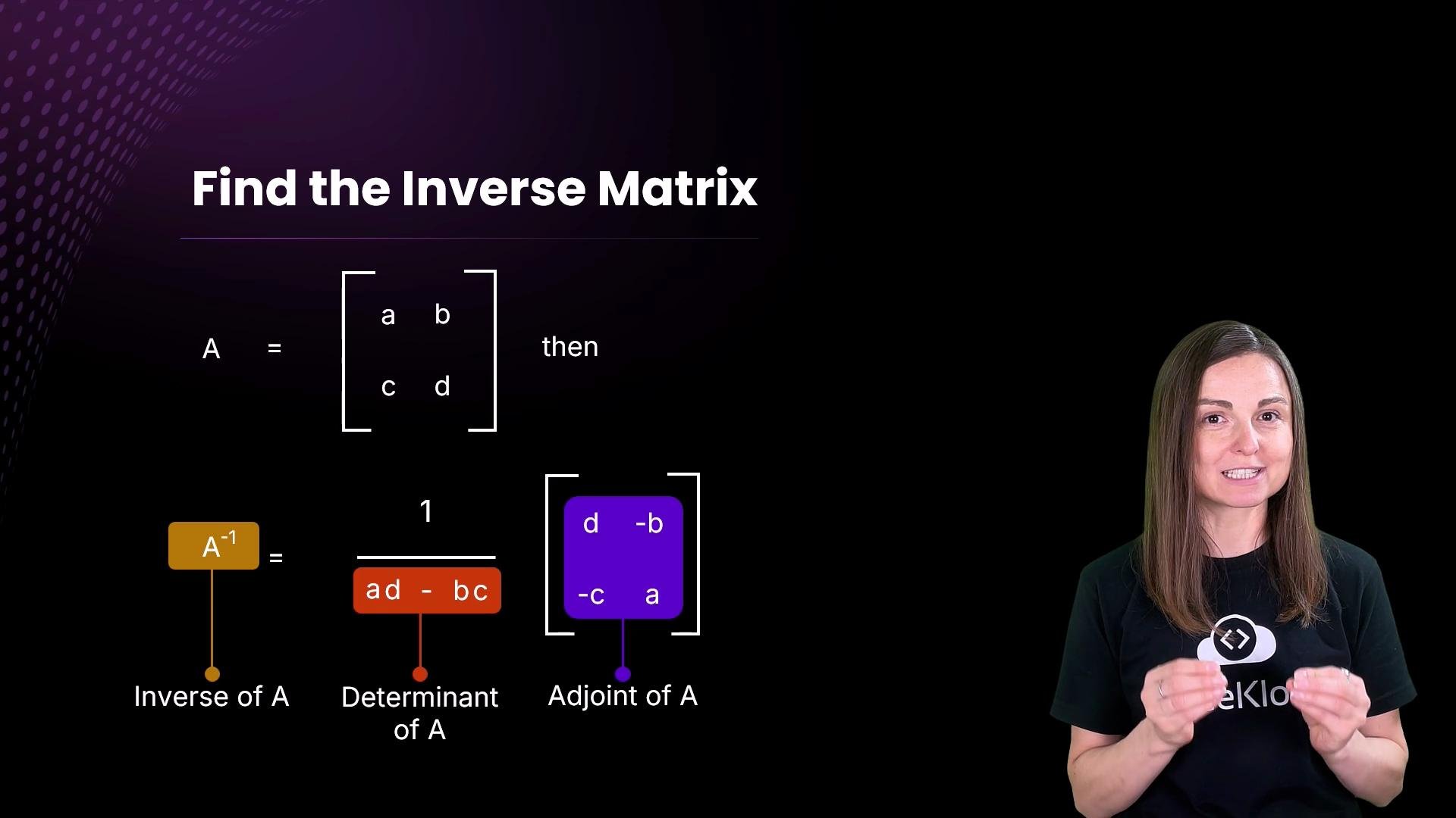
Formula for the inverse of a 2×2 matrix Given A: [ [a, b], [c, d] ] The inverse (when it exists) is: A^ = (1 / (ad − bc)) × adj(A) where:
  • ad − bc is the determinant of A.
  • adj(A) (the adjugate) is formed by swapping a and d, and negating b and c:
adj(A) = [ [ d, −b ], [ −c, a ] ]
The image explains how to find the inverse of a 2x2 matrix, showing the formula involving the determinant and adjoint. A person is also present, likely giving an explanation.
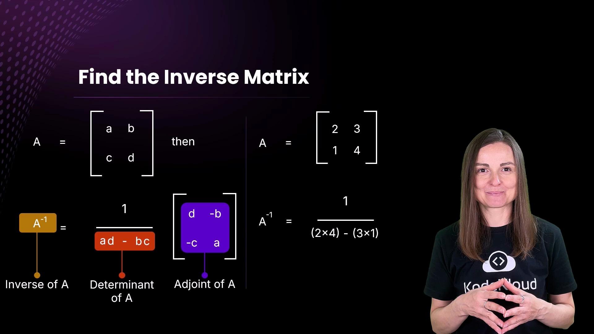
Step-by-step example Let A have entries a = 2, b = 3, c = 1, d = 4.
  1. Compute the determinant:
det(A) = ad − bc = 2×4 − 3×1 = 8 − 3 = 5
  1. Form the adjugate by swapping a and d and negating b and c:
adj(A) = [ [ 4, −3 ], [ −1, 2 ] ]
  1. Multiply the adjugate by 1/det(A):
A^ = (1/5) × [ [ 4, −3 ], [ −1, 2 ] ]
The image is a tutorial on finding the inverse of a 2x2 matrix, showing the formula and an example calculation. A woman stands to the right, gesturing with her hands.
Verify by multiplication To confirm A^ is correct, multiply A by A^ and check you get the identity matrix I = [ [1,0], [0,1] ]. Do the four scalar dot-products in the usual order:
  • row 1 of A × column 1 of A^
  • row 1 of A × column 2 of A^
  • row 2 of A × column 1 of A^
  • row 2 of A × column 2 of A^
Compute the raw products before scaling by 1/5, then apply the scalar factor:
  • (row1·col1) = 2×4 + 3×(−1) = 8 − 3 = 5
  • (row1·col2) = 2×(−3) + 3×2 = −6 + 6 = 0
  • (row2·col1) = 1×4 + 4×(−1) = 4 − 4 = 0
  • (row2·col2) = 1×(−3) + 4×2 = −3 + 8 = 5
Raw result matrix = [ [5, 0], [0, 5] ]. Multiplying by the scalar 1/5 gives I = [ [1,0], [0,1] ], confirming the inverse.

The image shows a mathematical matrix multiplication process with a result, alongside a person gesturing in front of a black background.
Why the determinant matters The determinant ad − bc appears in the denominator of the inverse formula. If the determinant is zero, the formula would divide by zero and no inverse exists. Such matrices are called singular or non-invertible. Example of a zero determinant: det = 2×6 − 4×3 = 12 − 12 = 0
If the determinant equals zero the matrix has no inverse. Such matrices are called singular.
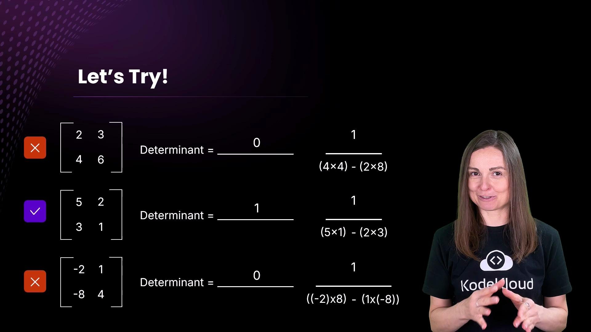
You can apply this determinant test to any small square matrix: only square matrices with nonzero determinant have inverses.
The image shows a presentation slide titled "Let's Try!" with matrices and their determinants, including checks and crosses indicating correctness. A person stands next to the slide, gesturing with their hands.
Quick reference table
ItemFormula / RuleNotes
Inverse (2×2)A^{-1} = (1/(ad-bc)) × [[d, -b], [-c, a]]Requires ad − bc ≠ 0
Determinant (2×2)ad − bcIf zero → singular (no inverse)
VerificationA × A^{-1} = IMultiply and check you get identity
Practical example: correcting sensor readings for movement Imagine sensor readings distorted by vehicle motion. The motion can be modeled by a movement matrix that transforms the true sensor matrix. To recover the original readings, multiply the measured sensor matrix by the appropriate correction matrix (the inverse of the movement matrix).
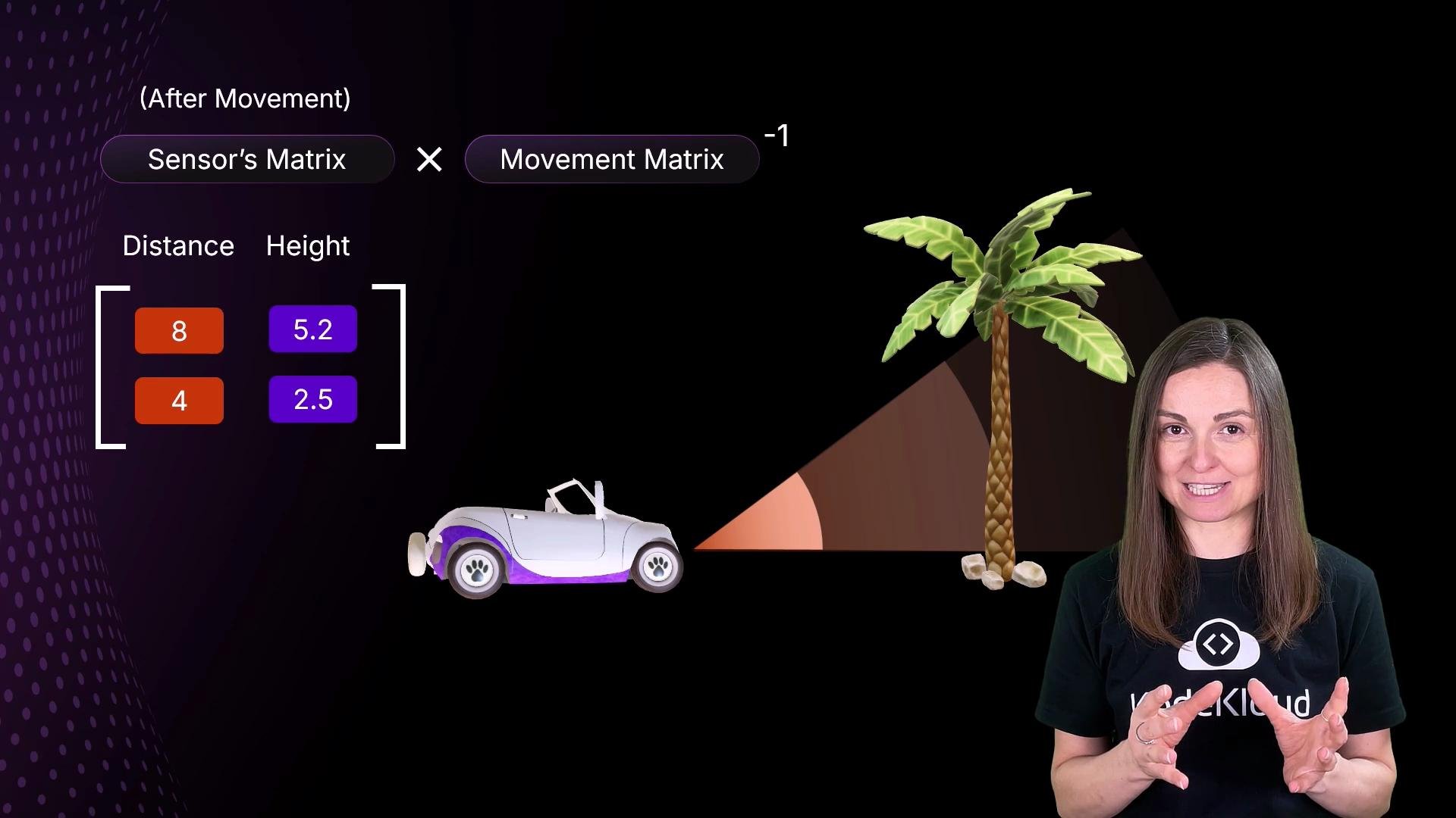
The image shows a woman in front of a graphical representation of a matrix calculation involving a car, a palm tree, and a cone of light. The matrix indicates "Distance" and "Height" values.
Apply the same inversion steps: compute (1/det) and the adjugate (swap a and d, negate b and c), then multiply that inverse by the sensor readings matrix to correct them.
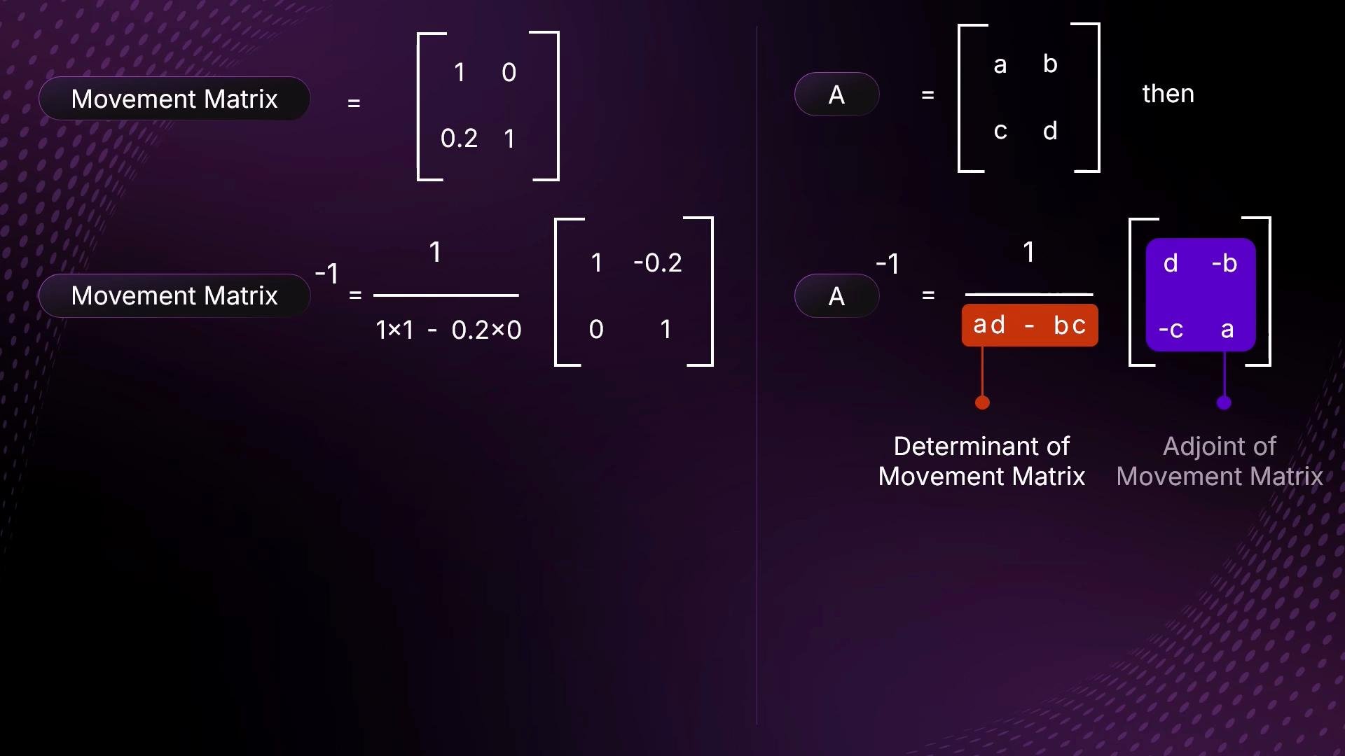
The image illustrates the calculation of the inverse of a 2x2 matrix, labeled as the "Movement Matrix," and explains the determinant and adjoint of the matrix.
After computing the inverse, multiply the sensor matrix by the correction matrix (again: row×column for each entry) and simplify to obtain corrected values.
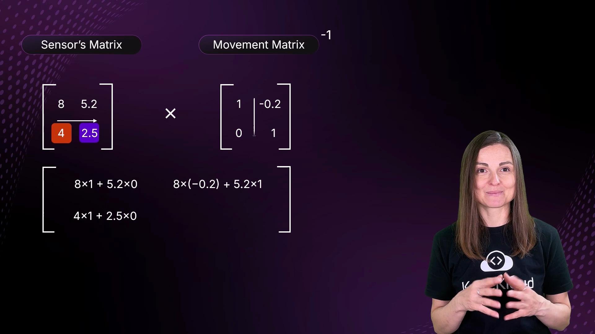
The image shows a mathematical problem involving matrix multiplication, labeled "Sensor's Matrix" and "Movement Matrix," with a person speaking or presenting in front of it. The background is a dark purple.
Compact example calculation
Sensor's Matrix
[ 8    5.2 ]
[ 4    2.5 ]

Movement Matrix (correction)
[ 1    -0.2 ]
[ 0     1   ]

Multiplication (Sensor × Movement)
[ 8×1 + 5.2×0    8×(-0.2) + 5.2×1  ]
[ 4×1 + 2.5×0    4×(-0.2) + 2.5×1  ]

Result
[ 8    3.6 ]
[ 4    1.7 ]
This small example shows how a correction (movement) matrix can restore readings closer to the intended values. In real systems, matrices are larger and numerically precise; matrix inversion and multiplication are central to sensor fusion, calibration, and real-time decision-making.
The image discusses the importance of matrices for self-driving cars, highlighting real-time decision-making and sensor data merging. A person is positioned in the lower right corner.
Summary
  • For a 2×2 matrix A = [ [a, b], [c, d] ], the inverse is A^{-1} = (1/(ad−bc)) × adj(A).
  • The determinant ad − bc must be nonzero for the inverse to exist.
  • Verification via A × A^{-1} = I confirms correctness.
  • Applications: inverse and multiplication are used for correcting sensor measurements, calibration, and many applied linear-algebra tasks in robotics and autonomous systems.
Further reading and references

Watch Video