

- Term frequency (TF)
- TF‑IDF (term frequency–inverse document frequency)
- Bag of words (BOW)
- TextRank
Term frequency (TF)
Term frequency quantifies how often a token appears inside a single document. It’s a simple and effective signal for identifying prominent words in a document. Example review: “excellent keyboard, excellent quality, excellent value”- Token counts:
excellent= 3,keyboard= 1,quality= 1,value= 1 - If the document has 6 tokens total, the term frequency for
excellentis 3 / 6 = 0.5.
count(t, d) is the number of occurrences of term t in document d, and |d| is the total number of terms in d.
Why use TF?
- Quick to compute and interpretable.
- Useful for surfacing frequent words in a document (e.g., common opinions in reviews).
- TF does not account for how common a term is across other documents, so very common words can appear important even if they are not discriminative.
TF‑IDF
TF‑IDF combines term frequency with inverse document frequency to highlight words that are frequent in a document but rare across the corpus. This helps surface terms that discriminate one document from many. Intuition:TFrewards high frequency in a document.IDFdownweights terms that appear in many documents.
N is the total number of documents and DF(t) is the number of documents that contain term t. TF‑IDF is typically computed as:
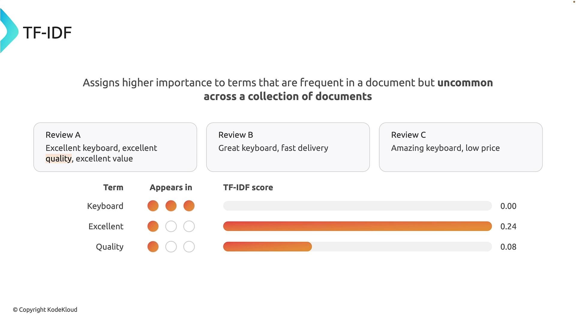
keyboard appears across many reviews, its IDF is low and the TF‑IDF score will be reduced; if excellent appears often in one review but not others, it receives a higher TF‑IDF score for that document.
TF‑IDF is a statistical importance score: it surfaces discriminative words but does not capture sentiment or semantic meaning. Use it for keyword extraction and as features for classical ML models.
Bag of words (BOW)
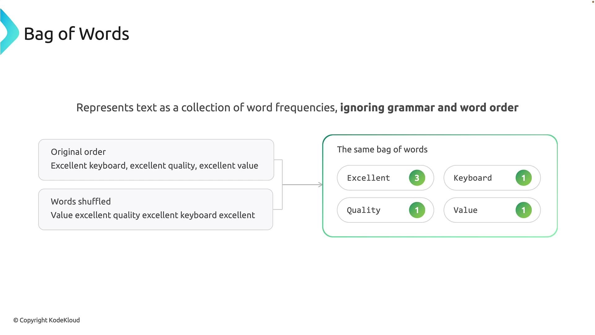
The bag-of-words model represents a document as a multiset of tokens and their counts. BOW discards word order and syntax—only token presence and frequency matter. Example:- Original: “excellent keyboard, excellent quality, excellent value”
- Bag-of-words:
excellent: 3, keyboard: 1, quality: 1, value: 1
- Simple and computationally efficient.
- Works well for many classic tasks such as document classification and spam detection.
- Loses word order and syntactic relations; cannot distinguish sentences that share the same words but have different meanings.
Bag-of-words discards order and grammatical relationships. Use it only when sequence and syntax are not important for the task.
TextRank
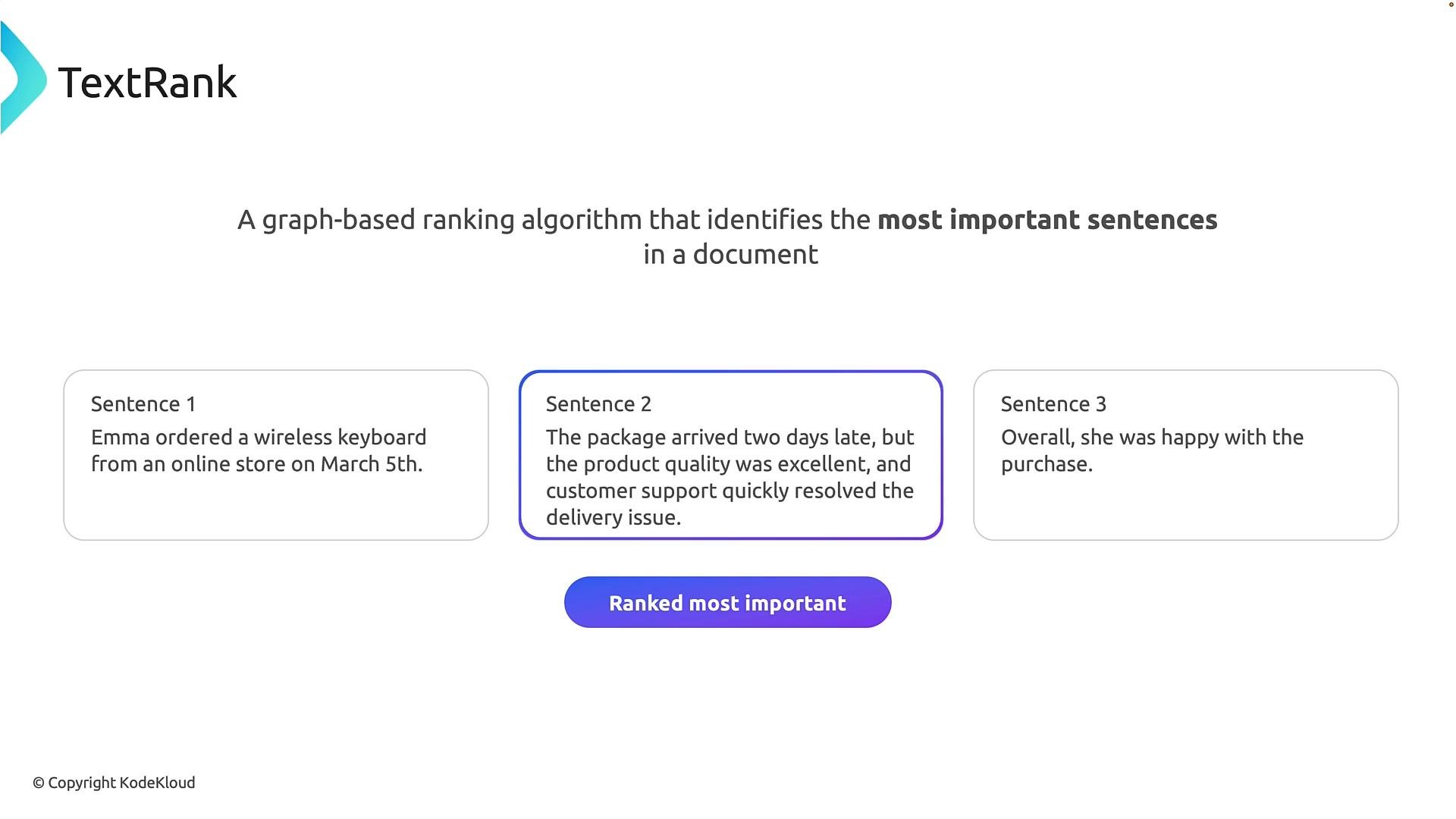
TextRank is a graph-based ranking algorithm that identifies the most important sentences for extractive summarization. It models sentences as nodes and connects them with edges weighted by similarity. Typical TextRank pipeline:- Tokenize the document into sentences (nodes).
- Compute pairwise similarity between sentences (edges), e.g., based on shared keywords, TF‑IDF vectors, or semantic embeddings.
- Run a PageRank-style algorithm to score sentences.
- Select the top-ranked sentences to build an extractive summary.
Summary comparison
These techniques provide complementary, measurable ways to represent text. They remain useful today as features for machine learning and as lightweight baselines before moving to semantic language models.
Links and references
- PageRank (Wikipedia)
- TF‑IDF in scikit-learn
- Introduction to Bag of Words (blog)
- TextRank paper and resources
- Gensim (topic modeling and TextRank-like utilities)