- What TF-IDF stands for and the role of each component.
- The core intuition: amplify words that are frequent inside a document and downweight words that appear across many documents.
- How TF-IDF is applied to rank documents for queries.
- A concise worked example with step-by-step calculations.
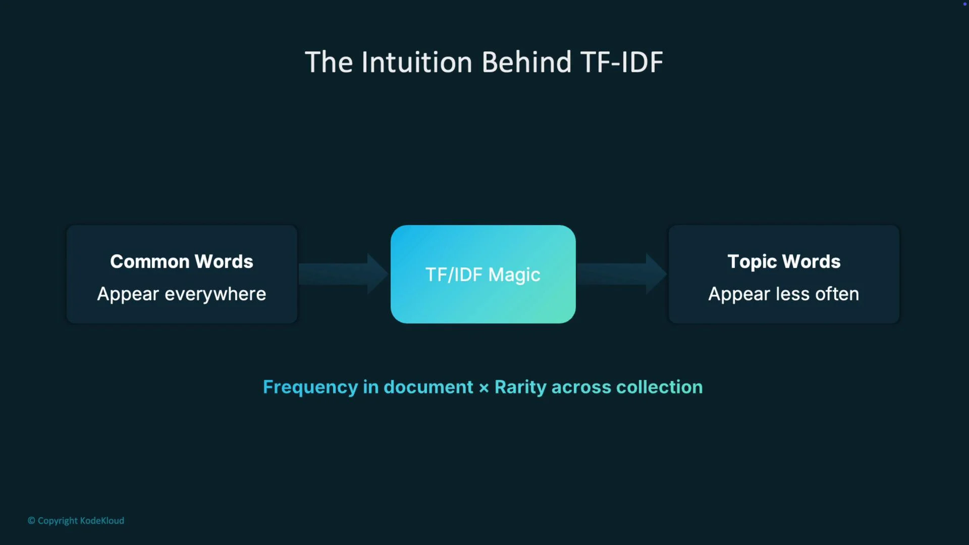
Intuition
Before jumping into formulas, consider how you naturally infer a document’s subject. You tend to ignore filler words like “the”, “and”, or “of” because they appear everywhere and don’t help identify topics. In contrast, specific terms such as “four-stroke”, “valve”, or “piston” strongly indicate the text is about engines. Those distinctive terms — and their co-occurrence patterns — provide the most informative cues.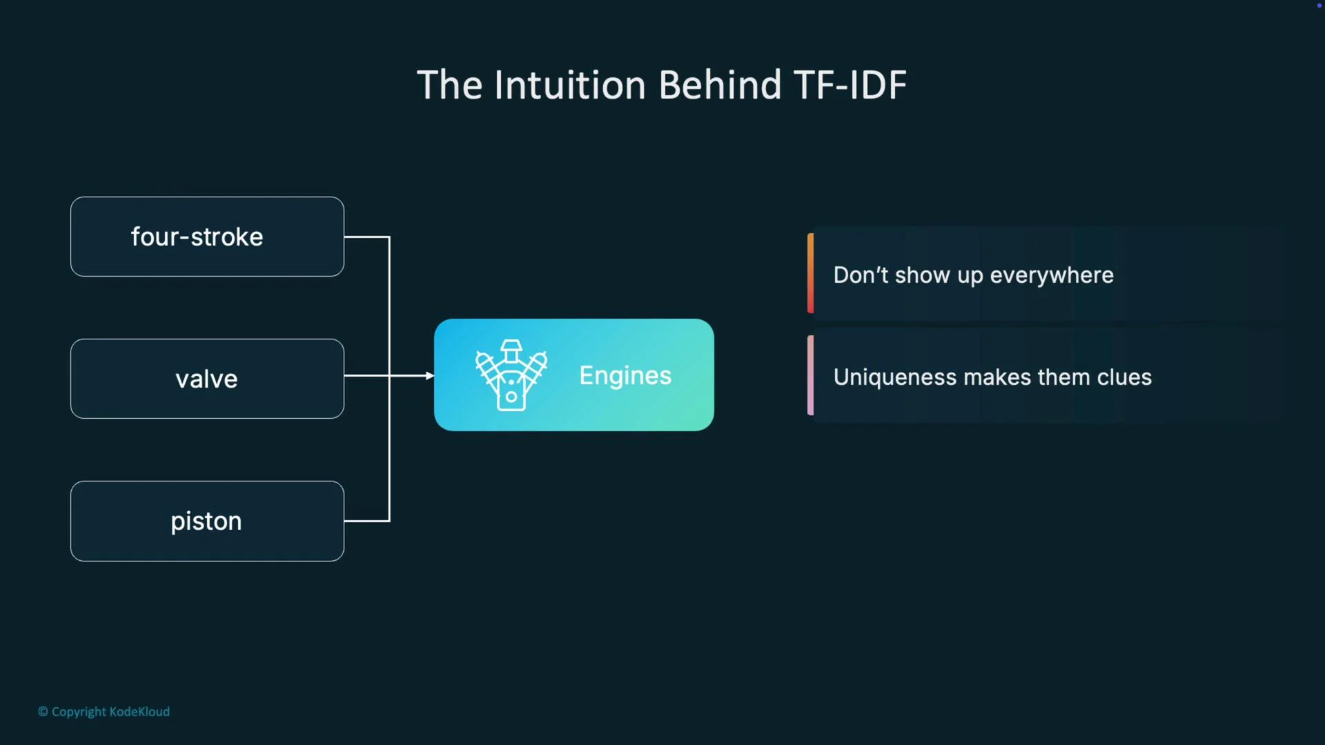
Pipeline overview
A typical TF-IDF ranking pipeline:- Receive the query terms.
- Tokenize the query and each document into terms.
- Count term occurrences per document and compute Term Frequency (TF).
- Compute Inverse Document Frequency (IDF) from how many documents contain each term.
- Multiply TF × IDF to obtain per-term weights.
- Sum the TF-IDF weights for the query terms in each document to produce a relevance score.
- Rank documents by that relevance score (highest first).
Term Frequency (TF)
Term Frequency measures how prominent a term is within a single document. Variants include:
A common normalized TF formula:
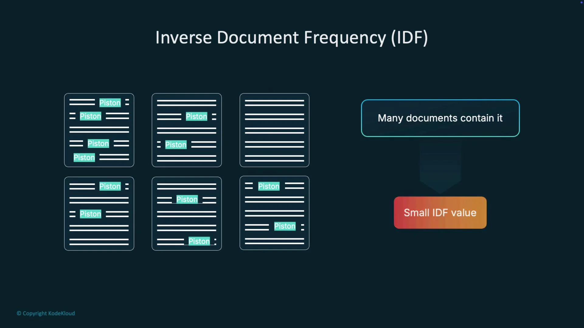
Inverse Document Frequency (IDF)
IDF measures how rare or common a term is across the whole collection. If a term appears in many documents, it is less useful for distinguishing them. Common IDF variants:
Example:
df_t is large (term appears everywhere), IDF is small. If df_t is small (term is rare), IDF is large. In production pipelines you usually remove very common stop words before scoring to avoid distorted IDF on small collections.
Combining TF and IDF
TF-IDF multiplies the two signals so that high scores require both within-document prominence and cross-document rarity: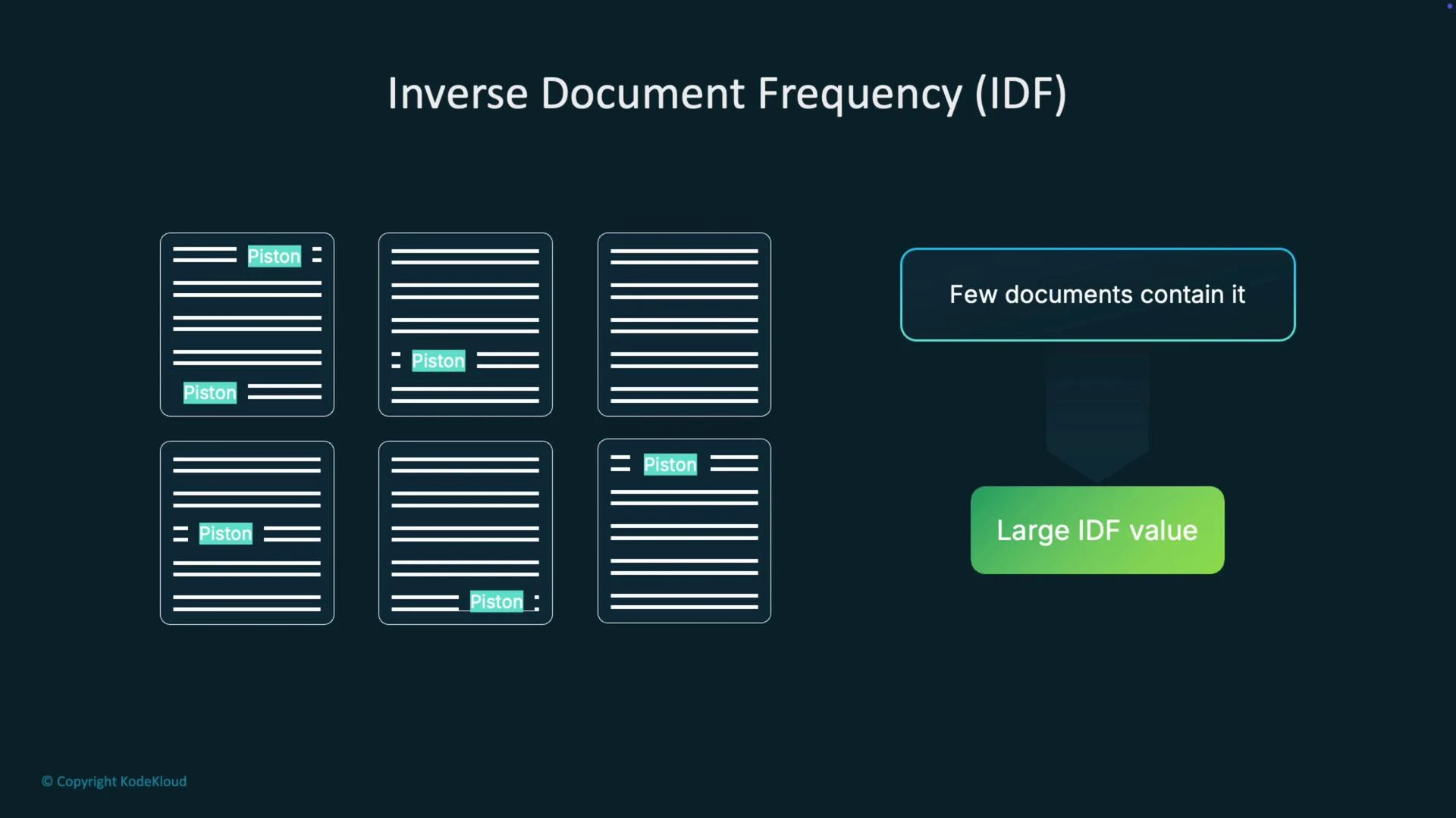
Worked example (step-by-step)
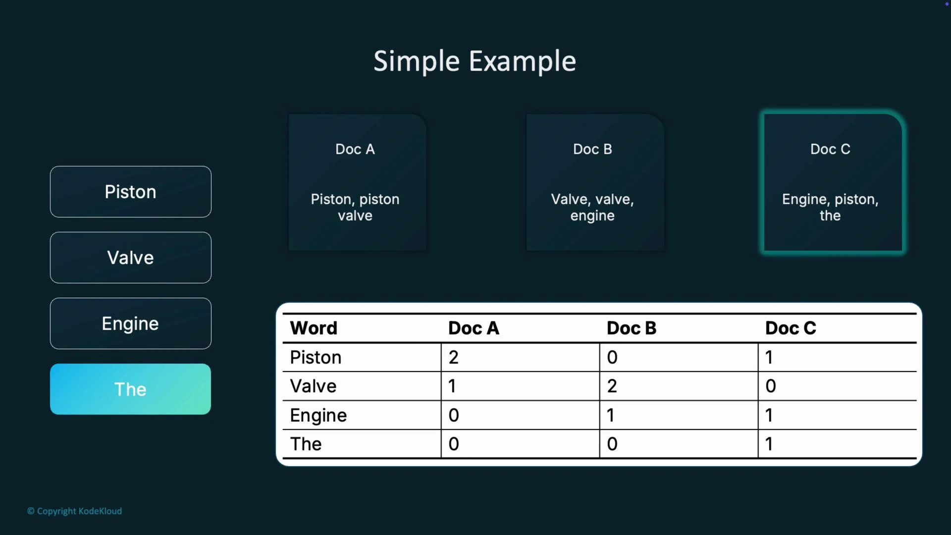
Three short documents:- Doc A: piston, piston, valve
- Doc B: valve, valve, engine
- Doc C: engine, piston, the
- Vocabulary:
piston,valve,engine,the - Document frequencies (df):
pistonappears in Doc A and Doc C →df_piston = 2valveappears in Doc A and Doc B →df_valve = 2engineappears in Doc B and Doc C →df_engine = 2theappears only in Doc C →df_the = 1
- Total documents:
N = 3
-
piston
- Doc A: TF = 2/3 ≈ 0.6667 → TF-IDF ≈ 0.6667 × 0.4055 ≈ 0.2703
- Doc B: TF = 0 → TF-IDF = 0
- Doc C: TF = 1/3 ≈ 0.3333 → TF-IDF ≈ 0.3333 × 0.4055 ≈ 0.1352
-
valve
- Doc A: TF = 1/3 ≈ 0.3333 → TF-IDF ≈ 0.1352
- Doc B: TF = 2/3 ≈ 0.6667 → TF-IDF ≈ 0.2703
- Doc C: TF = 0 → TF-IDF = 0
-
engine
- Doc A: TF = 0 → TF-IDF = 0
- Doc B: TF = 1/3 ≈ 0.3333 → TF-IDF ≈ 0.1352
- Doc C: TF = 1/3 ≈ 0.3333 → TF-IDF ≈ 0.1352
-
the
- Doc C: TF = 1/3 ≈ 0.3333 → TF-IDF ≈ 0.3333 × 1.0986 ≈ 0.3662
the appears in nearly every document and its IDF would be near zero; search pipelines typically remove common stop words before computing scores.
Query-dependent ranking
TF-IDF scores are computed per query term and summed to create a document score. For single-term queries:- Query “piston”: Doc A (0.2703) > Doc C (0.1352) > Doc B (0). Doc A ranks highest.
- Query “valve”: Doc B (0.2703) > Doc A (0.1352) > Doc C (0). Doc B ranks highest.
- Query “engine”: Doc B and Doc C tie (both ≈ 0.1352) and would be co-ranked unless tie-breaking rules apply.
Where TF-IDF is used
TF-IDF remains useful across many scenarios:- Classic search engines (historically a backbone of ranking).
- Automatic keyword extraction and tagging.
- Fast baselines for relevance: quick, interpretable signals that require no training.
- Document deduplication and near-duplicate detection via TF-IDF vectors and similarity measures (e.g., cosine similarity).
- Content analysis to surface themes and important terms across large corpora.
TF-IDF is fast, transparent, and requires no labeled training data. It’s especially effective when documents use distinctive vocabulary (for example, technical or legal texts) and when you need an interpretable baseline.
Limitations: TF-IDF has no semantic understanding (synonyms are distinct), ignores word order and context (bag-of-words), and is sensitive to corpus size and stop-word handling. Combine TF-IDF with embeddings or re-rankers when you need semantic relevance.
Limitations (expanded)
- No semantic similarity: synonyms and related concepts (e.g., “car” vs “automobile”) are treated as different tokens.
- Bag-of-words: ignores order and phrase structure (e.g., “dog bites man” ≠ “man bites dog”).
- Static and not adaptive: TF-IDF does not learn from user feedback unless combined with behavioral signals.
- Corpus sensitivity: small collections can give misleading IDF values for a few words.
- Stop-word handling: must filter or treat common words carefully to avoid noisy signals.
References and further reading
- TF-IDF — Wikipedia
- Khan Academy — Term Frequency–Inverse Document Frequency (introductory resources)
- Scikit-learn — Feature extraction text — practical implementation notes