Welcome back. In this lesson we demonstrate how text from a large PDF is converted into vector embeddings, stored in a vector database (ChromaDB), and visualized in 3D after dimensionality reduction. This walkthrough helps you understand how semantic similarity appears spatially when embeddings are projected to three principal components. What you’ll learn:
  • Extract text from a PDF and chunk it for embedding
  • Create embeddings with a sentence-transformer model
  • Persist embeddings and chunk metadata in ChromaDB
  • Retrieve embeddings, reduce dimensionality with PCA, and plot an interactive 3D scatter using Plotly
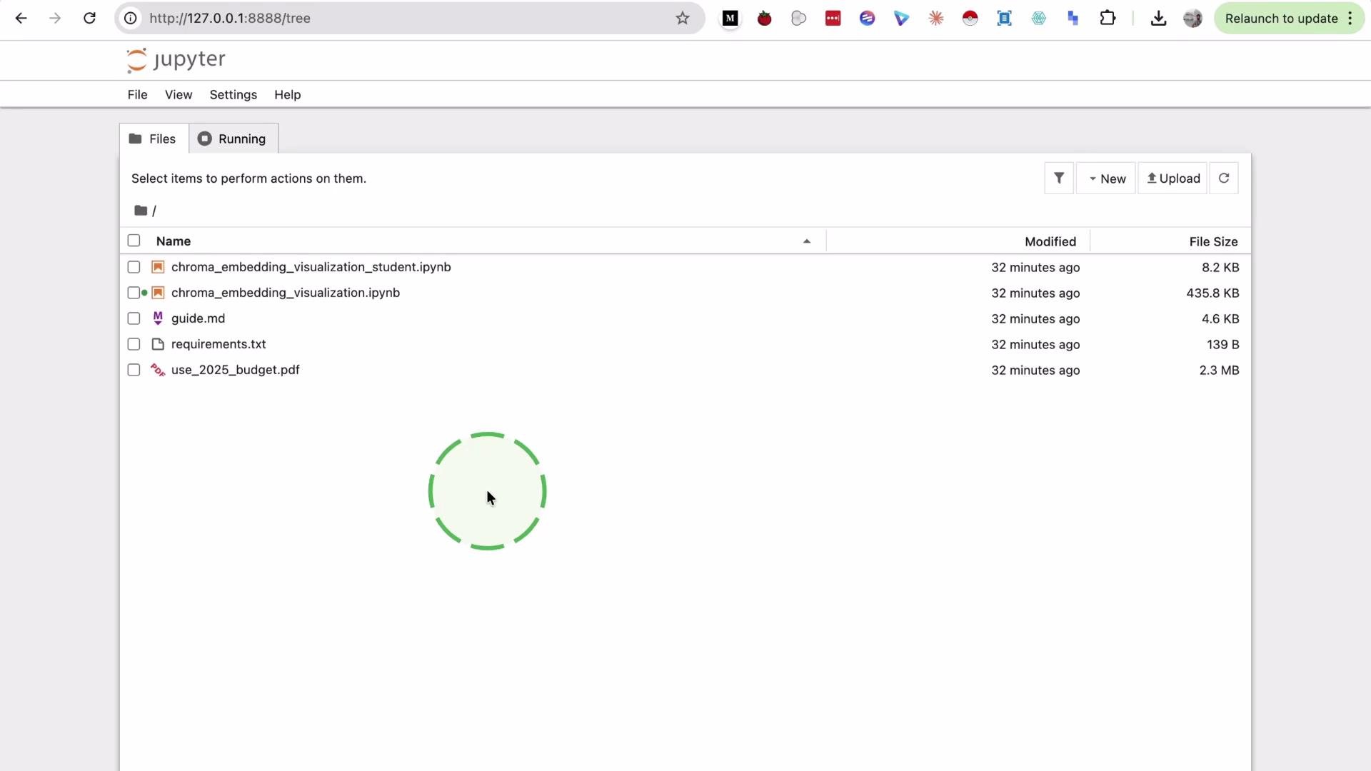
Let’s jump into the demo.
The image shows a Jupyter Notebook interface displaying a file directory, which includes various files like Jupyter notebooks, a markdown file, a requirements text file, and a PDF document.
Overview of the demo flow:
  1. Load a PDF document.
  2. Extract and split text into overlapping chunks.
  3. Embed each chunk with a sentence-transformer.
  4. Store embeddings and chunk text/metadata in ChromaDB.
  5. Retrieve embeddings, run PCA → 3 components.
  6. Render an interactive 3D Plotly scatter with chunk previews on hover.

The demo uses a large PDF (U.S. Government Budget FY 2025, ~188 pages) to illustrate how real-world documents produce many chunks and embeddings.
The image shows a digital PDF viewer open to the document "Budget of the U.S. Government, Fiscal Year 2025," displaying its cover page and thumbnails of the first few pages.
Required imports (run once at the top of the notebook)
# Python imports for the demo
import os
import numpy as np
import pandas as pd
import PyPDF2
import chromadb
from chromadb.utils import embedding_functions
from chromadb.config import Settings
from sklearn.decomposition import PCA
import plotly.express as px
Quick reference — key components used:
ComponentPurposeNotes / Example
PDF loaderExtract raw text from PDF pagesUses PyPDF2
ChunkingSplit text into overlapping segmentsConfigurable chunk_size and overlap
EmbeddingsConvert chunks to vectorsSentenceTransformerEmbeddingFunction(model_name="all-MiniLM-L6-v2")
Vector DBPersist vectors + metadatachromadb.PersistentClient(path="./chroma_data")
Dimensionality reductionProject to 3D for visualizationsklearn.decomposition.PCA(n_components=3)
VisualizationInteractive 3D scatter with previewsplotly.express.scatter_3d
  1. PDF loading function This function reads a PDF and concatenates all page text into a single string. It is robust to pages without extractable text.
def load_pdf_text(pdf_path: str) -> str:
    """
    Extract all text from a PDF file.

    Args:
        pdf_path: Path to the PDF file (e.g., 'use_2025_budget.pdf' or './01-vector-visualise/use_2025_budget.pdf')

    Returns:
        Concatenated text from all pages.
    """
    text_parts = []
    with open(pdf_path, "rb") as f:
        reader = PyPDF2.PdfReader(f)
        for page in reader.pages:
            text_parts.append(page.extract_text() or "")
    return "\n".join(text_parts)

print("✅ PDF loading function defined.")
  1. Chunking function We split the concatenated text into overlapping character-based chunks. Overlap preserves semantic continuity between adjacent chunks, which helps downstream tasks like retrieval and visualization.
def chunk_text(text: str, chunk_size: int = 500, overlap: int = 50) -> list[str]:
    """
    Split text into overlapping chunks.

    Args:
        text: Full document text.
        chunk_size: Maximum characters per chunk (default 500).
        overlap: Character overlap between consecutive chunks (default 50).

    Returns:
        List of text chunks.
    """
    if not text or not text.strip():
        return []

    chunks = []
    start = 0
    step = chunk_size - overlap
    while start < len(text):
        end = start + chunk_size
        chunk = text[start:end].strip()
        if chunk:
            chunks.append(chunk)
        start += step
    return chunks

print("✅ Chunking function defined.")
  1. ChromaDB setup and embedding function Create a persistent ChromaDB client that stores data on disk (./chroma_data). Configure the embedding function using the all-MiniLM-L6-v2 sentence-transformers model (compact and fast). The first run will download the model weights.
# ChromaDB client (persists to disk in ./chroma_data)
client = chromadb.PersistentClient(path="./chroma_data")

# Embedding function using sentence-transformers (all-MiniLM-L6-v2)
# First run: downloads ~90MB model and loads weights (may take 1-2 minutes)
print("Loading embedding model (all-MiniLM-L6-v2)...")
ef = embedding_functions.SentenceTransformerEmbeddingFunction(model_name="all-MiniLM-L6-v2")

# Create or get collection for our document chunks
collection_name = "doc_embeddings"
try:
    collection = client.get_collection(name=collection_name, embedding_function=ef)
    print(f"Using existing collection: {collection_name}")
except Exception:
    collection = client.create_collection(name=collection_name, embedding_function=ef)
    print(f"Created new collection: {collection_name}")

print("✔️ ChromaDB setup complete.")
We store each chunk as the document text (and optionally other metadata) alongside its embedding in the vector database. This lets the visualization show a text preview when you hover over a point.
First-time model download and building the embedding index can take time and disk space. Persisting to ./chroma_data helps avoid repeated downloads on subsequent runs.
  1. Load the PDF, chunk it, and add chunks to ChromaDB Load the PDF, create overlapping chunks, and insert them into the ChromaDB collection. The snippet below clears the collection before insertion — useful while iterating. Comment out the deletion code if you want to append instead.
# Path to PDF (example file baked into the notebook environment)
PDF_PATH = "use_2025_budget.pdf"

# Load PDF and extract text
full_text = load_pdf_text(PDF_PATH)
print(f"Loaded {len(full_text)} characters from PDF.")

# Chunk the text (500 chars per chunk, 50 char overlap)
chunks = chunk_text(full_text, chunk_size=500, overlap=50)
print(f"Created {len(chunks)} chunks.")

# Optional: clear existing data if re-running (comment out to append)
try:
    client.delete_collection(collection_name)
    collection = client.create_collection(name=collection_name, embedding_function=ef)
except Exception:
    # If deletion fails (e.g., collection doesn't exist), continue
    pass

# Prepare IDs and metadata (index + preview)
ids = [f"chunk_{i}" for i in range(len(chunks))]
metadatas = [
    {"chunk_index": i, "preview": chunk[:80] + "..." if len(chunk) > 80 else chunk}
    for i, chunk in enumerate(chunks)
]

# Add chunks to ChromaDB (documents stored alongside embeddings)
collection.add(
    documents=chunks,  # stored as the document text for each item
    ids=ids,
    metadatas=metadatas
)

print(f"Added {len(chunks)} chunks to ChromaDB collection '{collection_name}'.")
Note: For a long PDF (188 pages) you may generate hundreds or thousands of chunks depending on chunk_size and overlap. Adjust chunking parameters to balance granularity and index size.
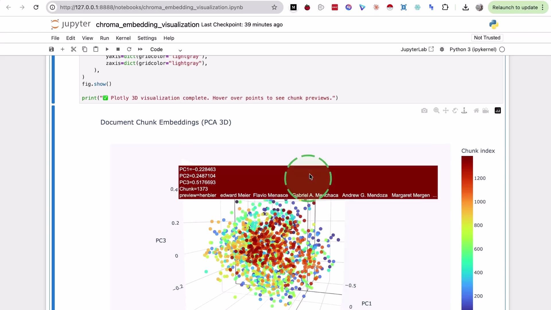
  1. Retrieve embeddings and visualize (PCA → 3D scatter) Query the collection to fetch embeddings and metadata, reduce dimensionality with PCA to three components, and render an interactive 3D scatter using Plotly. Hovering shows chunk previews stored in the collection.
# Fetch embeddings, documents, and metadata from ChromaDB
results = collection.get(include=["embeddings", "documents", "metadatas"])
embeddings = np.array(results["embeddings"])
documents = results["documents"]
metadatas = results["metadatas"] or [{}] * len(documents)

# PCA: reduce embedding dimensionality (e.g., 384D -> 3D)
pca = PCA(n_components=3)
reduced = pca.fit_transform(embeddings)

# Build DataFrame for Plotly visualization
df = pd.DataFrame({
    "x": reduced[:, 0],
    "y": reduced[:, 1],
    "z": reduced[:, 2],
    "chunk_index": [m.get("chunk_index", i) for i, m in enumerate(metadatas)],
    "preview": [doc[:200] + "..." if len(doc) > 200 else doc for doc in documents],
})

# Interactive 3D scatter - color by chunk index (continuous colormap)
fig = px.scatter_3d(
    df,
    x="x",
    y="y",
    z="z",
    color="chunk_index",
    color_continuous_scale="Turbo",
    hover_data=["chunk_index", "preview"],
    title="Document Chunk Embeddings (PCA 3D)",
    labels={"x": "PC1", "y": "PC2", "z": "PC3", "chunk_index": "Chunk"},
)

fig.update_traces(marker=dict(size=5, opacity=0.85, line=dict(width=0)))
fig.update_layout(
    template="plotly_white",
    height=650,
    coloraxis_colorbar=dict(title="Chunk index"),
    scene=dict(
        bgcolor="rgb(248, 248, 252)",
        xaxis=dict(gridcolor="lightgray"),
        yaxis=dict(gridcolor="lightgray"),
        zaxis=dict(gridcolor="lightgray"),
    ),
)

fig.show()
print("✔️ Plotly 3D visualization complete. Hover over points to see chunk previews.")
The interactive plot displays each chunk as a point in 3D space (PCA-reduced). Hover to view the chunk index and a brief text preview pulled from the collection.
The image shows a Jupyter Notebook interface displaying a 3D plot of document chunk embeddings using PCA, with color-coded points representing chunk indices.
What this visualization reveals
  • Each point corresponds to a text chunk’s embedding; embeddings encode semantic meaning.
  • PCA compresses high-dimensional vectors to three principal components so you can visually inspect structure.
  • Nearby points indicate semantically similar chunks; distant points indicate dissimilar content.
  • Storing chunk text as document/metadata lets you validate what each point represents during exploration.
A few important clarifications
  • Vector databases store embeddings (vectors). In this demo we intentionally store the chunk text alongside embeddings so the visualization can display previews — many vector DBs support this pattern.
  • Dimensionality reduction (PCA, t-SNE, UMAP) is only used for visualization; original vectors remain high-dimensional in the database and should be used for real retrieval tasks.
  • Visual clusters are a qualitative tool to inspect semantic grouping and to debug embedding/model behavior.
Further reading and references That concludes this demo on visualizing vectors stored in a vector database (ChromaDB). You should now have a clear example of how document text is converted into embeddings and how those vectors can be explored visually. See you in the next lesson.

Watch Video

Practice Lab