

- HNSW is conceptually similar to a skip list: a hierarchy of layers where upper layers are sparse and lower layers are increasingly dense.
- Upper layers provide long-range shortcuts for coarse navigation across the embedding space.
- The bottom layer (level 0) contains all vectors and dense local links for precise nearest-neighbor retrieval.
- Top layers: very sparse, long-range links — fast coarse jumps.
- Middle layers: intermediate connectivity — guide search toward the target region.
- Bottom layer: dense connectivity with all points — final fine-grained search.
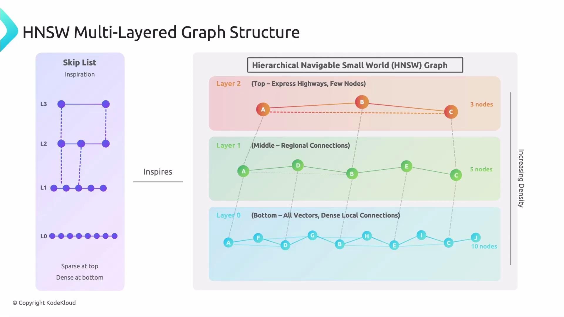
- Entry points at the top layer let you quickly traverse large distances in vector space.
- Each lower layer adds more nodes and more local edges, increasing search accuracy as you descend.
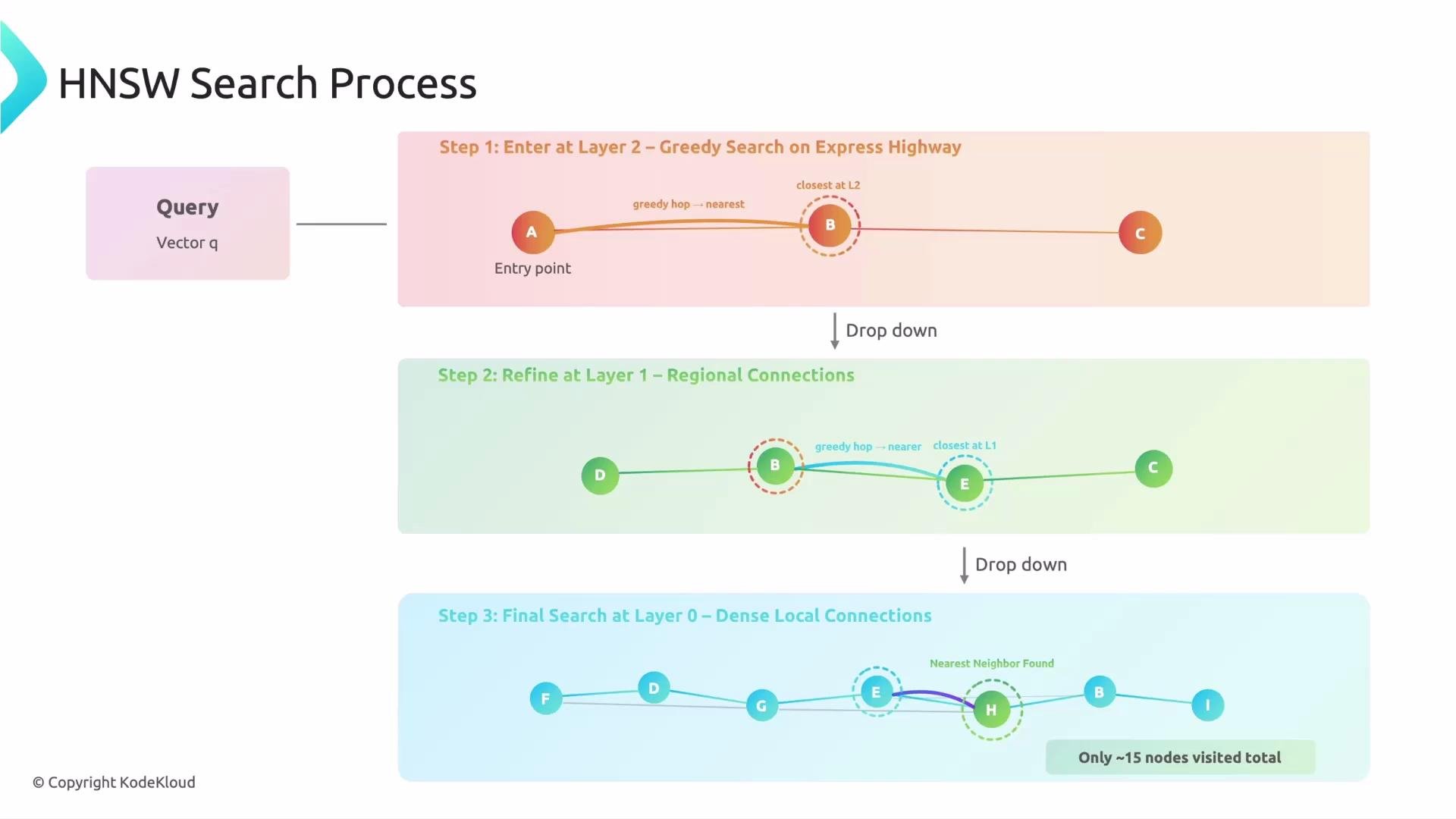
- The algorithm transitions from coarse to fine search: greedy climbs on sparse layers, and a more exhaustive candidate expansion on the bottom layer.
- Provide a query vector and start from an entry point at the highest layer.
- At each upper layer, perform greedy hill-climbing: repeatedly move to the neighbor that reduces distance to the query until no neighbor is closer. The goal is coarse localization.
- Take the best point found in the current layer as the entry point into the next (denser) layer.
- Repeat the greedy descent until reaching level 0 (the bottom layer).
- At level 0, perform a best-first (priority queue) search controlled by
ef(often calledefSearch) to collect the final k nearest neighbors.
efSearch.
HNSW is an approximate nearest neighbor algorithm. The most commonly tuned values are
M, efConstruction, and efSearch. Adjust these to balance recall, query latency, and memory. For production, benchmark recall vs latency for representative queries and vectors.- Index construction: increase
efConstructionandMif you need higher recall, especially for large or highly clustered datasets. Expect longer build times and higher memory use. - Query tuning: raise
efSearchto improve recall for difficult queries; lower it to reduce latency when recall requirements are modest. - Memory vs performance: higher connectivity (
M) and larger dynamic lists require more memory. Monitor memory consumption on nodes that host the index. - Entry point strategy: most implementations pick a randomized or high-degree node as entry. Consistent entry strategies help with predictable latency.
- Parallelism: many HNSW libs support parallel index building and multi-threaded searching — use available cores carefully for a production workload.
- Malkov, Y. A., & Yashunin, D. A. (2018). Efficient and robust approximate nearest neighbor search using Hierarchical Navigable Small World graphs (HNSW). Original HNSW paper
- Faiss — Facebook AI Similarity Search
- nmslib — Similarity Search library