

Brute-force (linear scan)
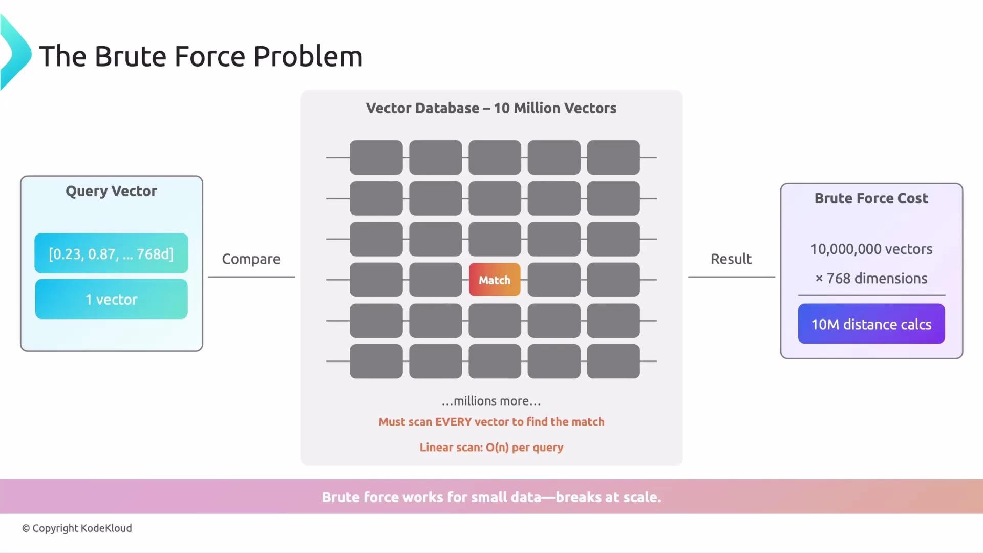
Brute force, or a linear scan, is the simplest way to run a nearest-neighbor search:- You submit a query vector (for example,
[0.23, 0.87, ...]in 768 dimensions). - The system compares that query against every vector stored in the database.
- If the database contains 10 million vectors, the system makes 10 million distance calculations per query, one-by-one, to find the closest matches.
Indexing to the rescue
Indexing is the set of techniques that let you avoid examining every vector. A simple analogy is a library:- Without an index, you open every book on every shelf until you find the one you want (linear scan).
- With an index (catalog), you look up the catalog, go to the right section, and search only a small subset of books.
Indexing typically uses Approximate Nearest Neighbor (ANN) techniques to deliver sublinear query latencies in large vector collections. This commonly trades a tiny amount of recall for orders-of-magnitude improvements in throughput and cost.
Complexity and trade-offs
- Linear scan: typically O(N × D) per query.
- Index-based search: can achieve sublinear behavior in N for many workloads; some structures aim for ~O(log N) under ideal conditions, but real-world performance depends on the algorithm, implementation, and data dimensionality.
High dimensional vectors (very large D) can reduce the effectiveness of many indexes. Always benchmark with your data distribution and query patterns—synthetic tests can be misleading.
Common ANN approaches
Here’s a concise comparison of standard ANN techniques and where they shine:
For more in-depth reading:
- HNSW paper and implementations
- Overview of Product Quantization
- Locality-Sensitive Hashing (LSH) concepts
Practical guidelines
- Start with a baseline: measure brute-force latency and recall to understand performance targets.
- Profile your data: dimensionality, sparsity, and cluster structure affect index choice.
- Benchmark multiple index types using realistic query loads and realistic candidate set sizes.
- Consider hybrid approaches: graph indices combined with quantization or inverted lists scale well in production.
- Monitor recall/precision trade-offs: tune index parameters (e.g., number of probes, ef/search size) to meet application SLAs.
Summary
- Brute force performs a full linear scan and becomes impractical as N grows.
- Indexing provides a catalog-like shortcut to inspect only a small region of relevant vectors.
- ANN indexes (graph-based, hashing, trees, quantization) are the practical solution for scalable vector search. Each offers trade-offs between speed, memory, build time, and accuracy—benchmark with your real data.