- Min–Max scaling (feature-wise)
- Normalization (row-wise / unit norm)
- Standardization (z-score, feature-wise)
- Algorithms that rely on distances (k-NN, k-means, SVM) or gradient-based optimization often perform better when features are on similar scales.
- Without scaling, a feature with large numeric values (e.g., house size in square feet) can dominate another feature with smaller numeric ranges (e.g., number of bedrooms), even if both are equally informative.
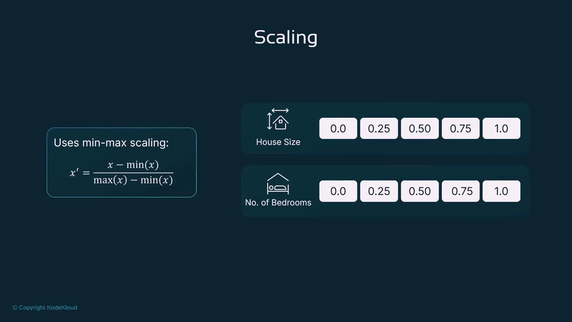
Min–Max Scaling (Feature-wise)
Min–Max scaling rescales each feature independently to a fixed range, typically [0, 1]. This preserves the relationships among the original values but bounds them.- Formula: x’ = (x − min(x)) / (max(x) − min(x))
- Operates column-wise (feature-wise)
- Use case: When you need bounded inputs or your algorithm is sensitive to absolute value ranges (k-NN, SVM, neural networks with activation functions)
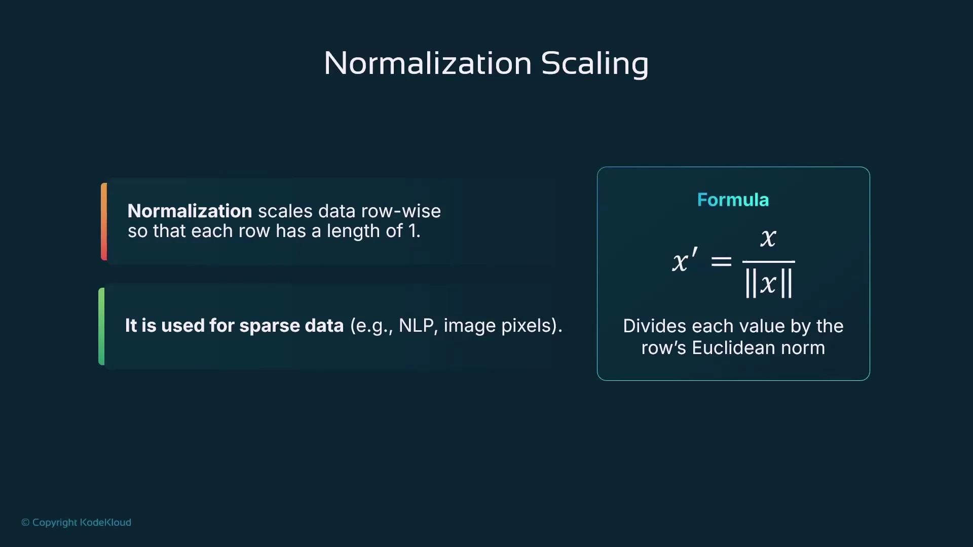
Normalization (Row-wise, Unit Norm)
Normalization rescales each sample (row) to unit length (norm = 1). This is a row-wise operation and is useful when vector direction matters more than magnitude — for example, cosine-similarity comparisons in NLP or when working with TF-IDF vectors.- Formula: x’ = x / ||x|| where ||x|| is typically the Euclidean (L2) norm
- Operates row-wise (sample-wise)
- Use case: Sparse data, text (TF-IDF), or any vector-space model where magnitude is irrelevant and only direction matters
- For a row [200000, 3], the L2 norm is sqrt(200000^2 + 3^2) ≈ 200000.x
- Dividing each element by that norm produces a unit-length vector (sum of squared components = 1)
Normalization is not the same as min–max scaling. Normalization rescales rows (samples) to unit length; min–max rescales features (columns) to a fixed range.
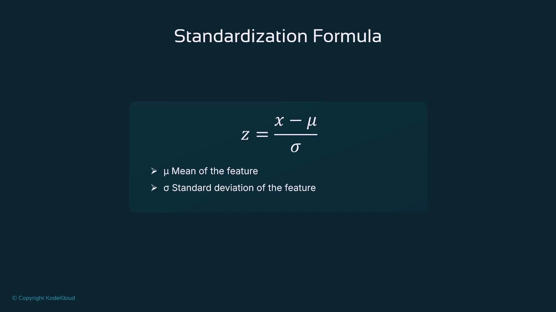
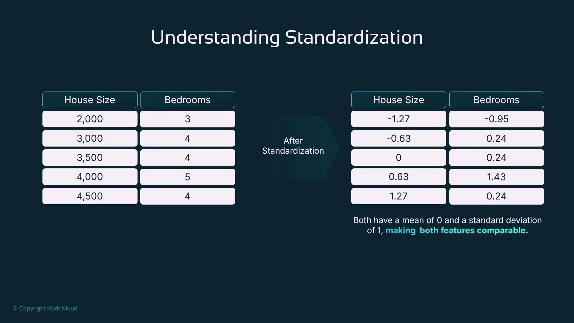
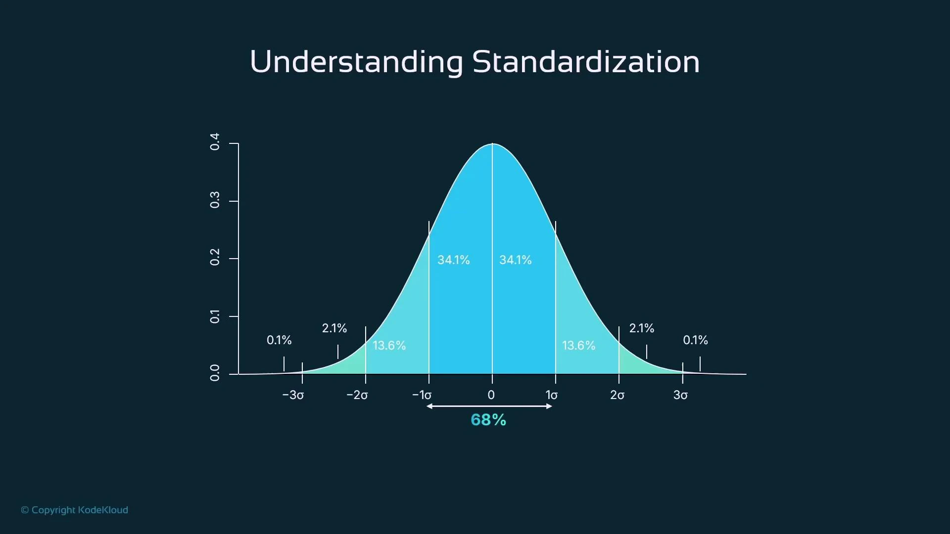
Standardization (Z-score, Feature-wise)
Standardization centers each feature on zero mean and scales to unit variance. This is a column-wise transformation and is often the default preprocessing for many statistical and machine learning algorithms.- Formula: z = (x − μ) / σ where μ is the feature mean and σ is the feature standard deviation
- Operates column-wise (feature-wise)
- Use case: Models that assume centered inputs or benefit from normalized variance (linear/logistic regression, SVM, PCA, gradient-based methods)
- Improves convergence for gradient-based optimizers
- Prevents features with larger numeric scales from dominating models
- Makes feature variances comparable
- For approximately normal features: ~68% of values fall within ±1σ, ~95% within ±2σ, and ~99.7% within ±3σ.
- Centering helps many algorithms behave more predictably and improves numerical stability.

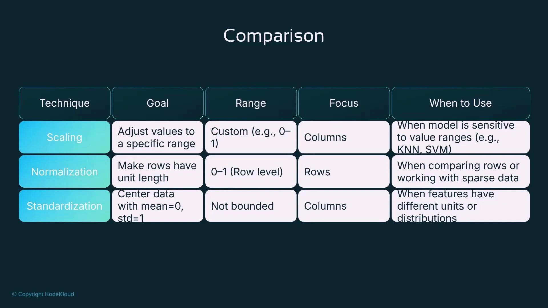
Quick Comparison: Scaling vs Normalization vs Standardization
| Method | Goal | Focus | Output Range | When to use | ||||
|---|---|---|---|---|---|---|---|---|
| Min–Max Scaling | Rescale features to a fixed range | Column-wise (feature) | Bounded, typically [0, 1] | When bounded inputs are required or for algorithms sensitive to absolute ranges (k-NN, SVM, neural nets) | ||||
| Normalization (Unit norm) | Scale each sample to unit length ( | x | = 1) | Row-wise (sample) | Usually values in [0,1] for non-negative data; interpreted as direction | For sparse or text data (TF-IDF) and when cosine similarity/direction matters | ||
| Standardization (Z-score) | Center features to mean 0 and scale to unit variance | Column-wise (feature) | Unbounded, usually within a few σ of mean | For algorithms that assume centered inputs or use variance information (linear/logistic regression, SVM, PCA) |
Summary & Recommendations
- Choose Min–Max scaling when you need bounded features (0–1) or are feeding values to models sensitive to absolute ranges.
- Use Normalization (unit norm) when working with sparse vectors or text (TF-IDF), and when only vector direction matters.
- Prefer Standardization for algorithms that assume zero-mean or when stabilizing and speeding up gradient-based training.
- scikit-learn: MinMaxScaler
- scikit-learn: Normalizer
- scikit-learn: StandardScaler
- Kubernetes Basics — for related deployment examples (if deploying models)