- Machine learning models require numeric input.
- Different encoding strategies introduce different assumptions (e.g., order vs. independence).
- Choosing the right encoding affects model performance, dimensionality, and risk of leakage.
Label encoding
Label encoding assigns a unique integer to every category in a feature. Consider aNeighborhood feature with values “Downtown”, “Suburbs”, and “Rural”. Label encoding might map these to 1, 2, and 3 respectively:
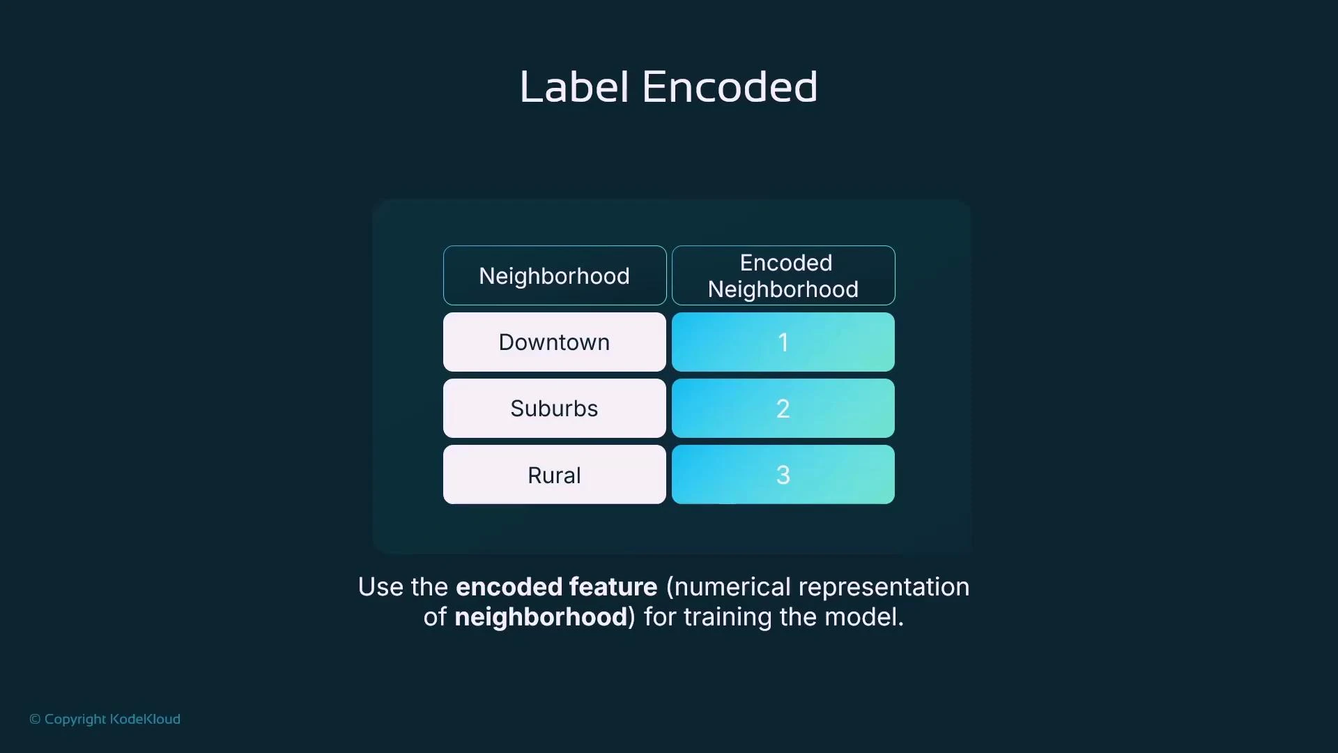
- Downtown → 1
- Suburbs → 2
- Rural → 3
- Simple and compact (single column).
- Imposes an ordinal relationship (1 < 2 < 3) that may not be meaningful. Models could interpret the numeric order as a ranking or distance, biasing predictions.
- When the categorical variable is ordinal (has a meaningful order), or when the algorithm you use can handle nominal labels without misinterpreting ordering.
One-hot encoding
To avoid introducing a false order, one-hot encoding creates binary indicator columns (flags) for each category. ForNeighborhood you would create Neighborhood_Downtown, Neighborhood_Suburbs, and Neighborhood_Rural. Each row has a 1 for the category it belongs to and 0 for the others. After adding the new columns you drop the original categorical column.
Example using scikit-learn:
- One-hot encoding removes implied order by creating independent binary features.
- It expands the feature space — each unique category becomes a column.
Use one-hot encoding for nominal categorical variables (no natural order). Be mindful that one-hot can significantly increase dimensionality when the category count grows.
High cardinality and the downside of one-hot encoding
One-hot encoding works well for low-cardinality features, but when a categorical feature has many unique values (high cardinality) it produces a wide, sparse dataset. This can increase model complexity, memory usage, and training time without improving predictive power—especially for features such as postcodes, user IDs, or product SKUs.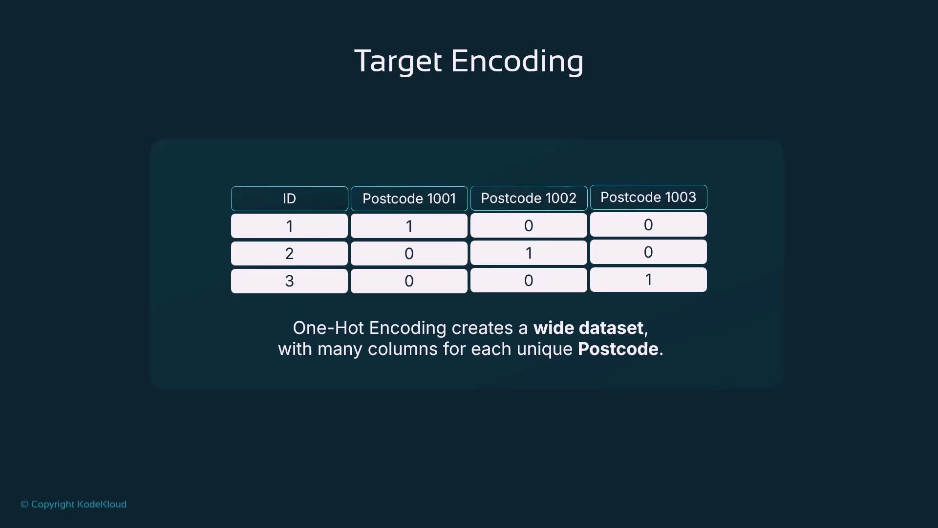
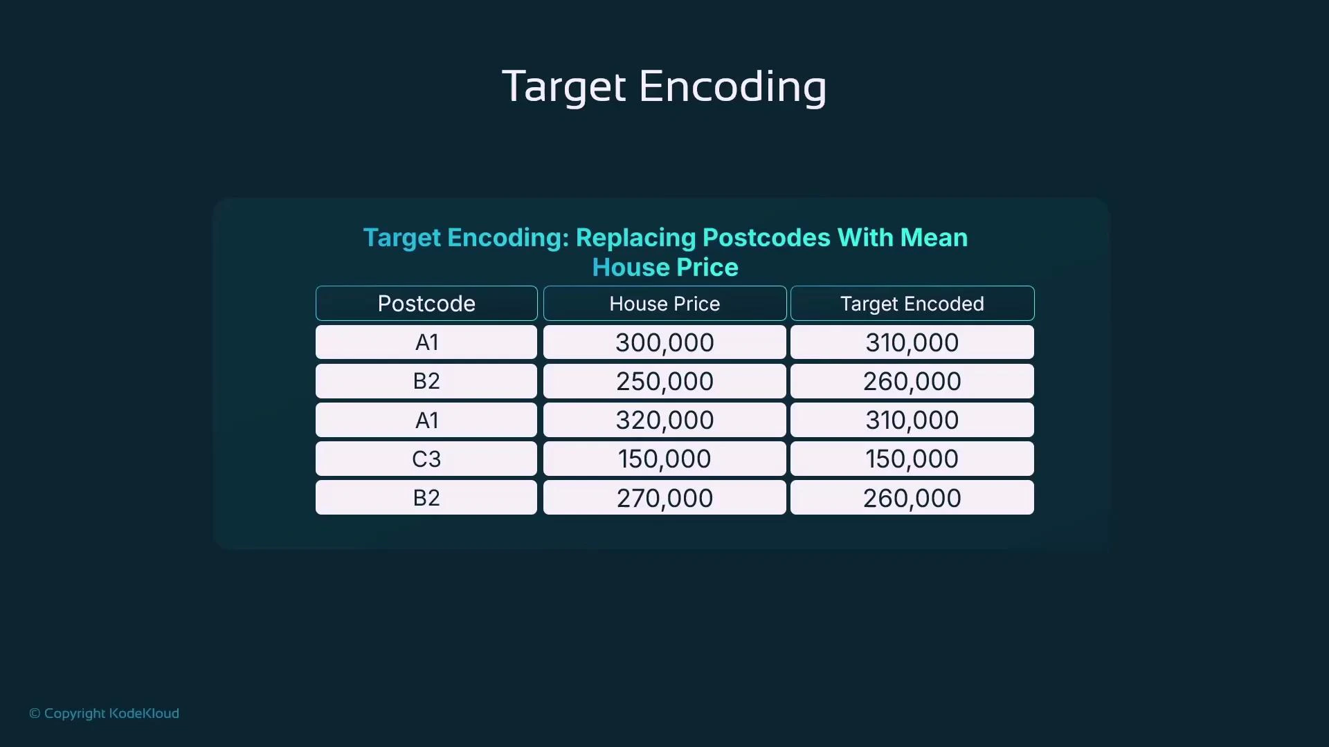
Target encoding (mean encoding)
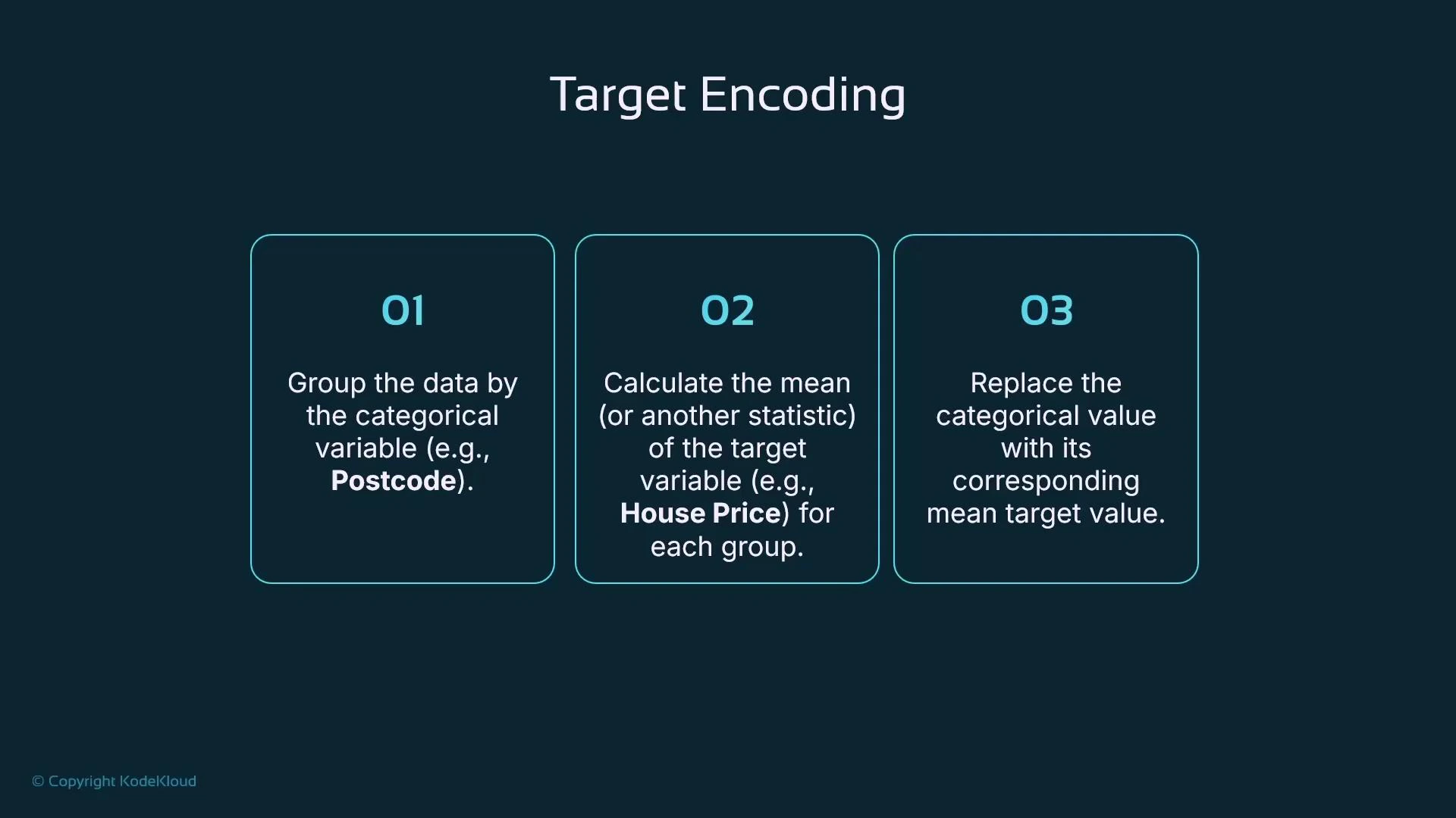
Target encoding replaces each category with a statistic of the target variable computed over that category—most commonly the mean target value. This reduces dimensionality while preserving the relationship between the categorical feature and the target. Typical steps:- Group data by the categorical variable (e.g., postcode).
- Compute the mean (or other statistic) of the target for each group.
- Replace the categorical value with that statistic.
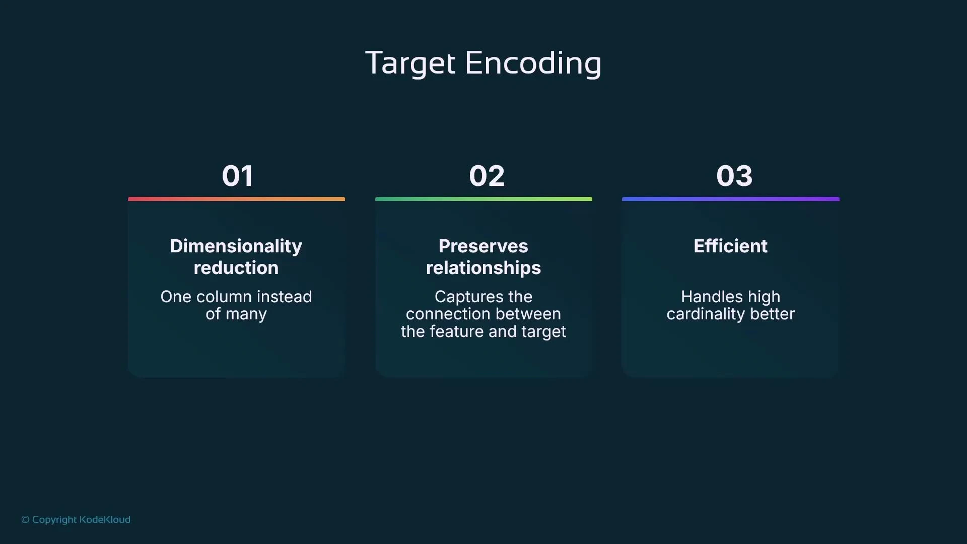
- Dimensionality reduction: one numeric column instead of many indicator columns.
- Preserves a relationship between the categorical feature and the target.
- Efficient for high-cardinality features.
- Compute the mean house price per postcode.
- Substitute that mean as the encoded value for every row with that postcode.
- Smoothing: combine per-category statistics with the global statistic to reduce variance for rare categories.
- Handling unseen categories: use a global mean or a special fallback value.
- Use regularization or weight by category size to prevent noisy estimates from small groups.
Target encoding can leak target information if applied naively (computing encodings on the full dataset). Prevent leakage using out-of-fold (cross-validated) encodings, train-only computations, or smoothing techniques.
Quick comparison of encoding strategies
| Encoding method | Best for | Pros | Cons |
|---|---|---|---|
| Label encoding | Ordinal categories | Compact, simple | Imposes order that may be meaningless |
| One-hot encoding | Low-cardinality nominal categories | No implicit order, interpretable | Can explode feature space for high cardinality |
| Target encoding | High-cardinality categories correlated with target | Compact, captures target relationships | Risk of target leakage, needs smoothing/out-of-fold schemes |
Summary / Practical checklist
- Outliers: detect with methods like IQR; decide whether to drop, cap (Winsorize), or otherwise transform them.
- Scaling: pick scaling appropriate to model type — standardization (zero mean, unit variance), min-max scaling, or normalization (e.g., L2) for distance-based methods.
- Categorical data: convert categories to numeric values using an encoding strategy that matches the data and model:
- Label encoding for ordinal categories.
- One-hot encoding for low-cardinality nominal features.
- Target encoding (with out-of-fold or smoothing) for high-cardinality features.
- Avoid leakage: never compute encodings on the full dataset before splitting; use cross-validation/out-of-fold approaches.
- Tools: use libraries like pandas, NumPy, and scikit-learn for preprocessing tasks.