- What training data must contain.
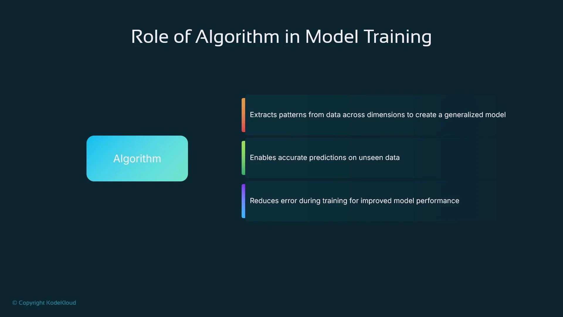
- How an algorithm creates a model artifact from data.
- How inference works on a hosted prediction endpoint.
- The math behind linear regression and loss minimization.
- How training generalizes to multiple features and the risk of overfitting.
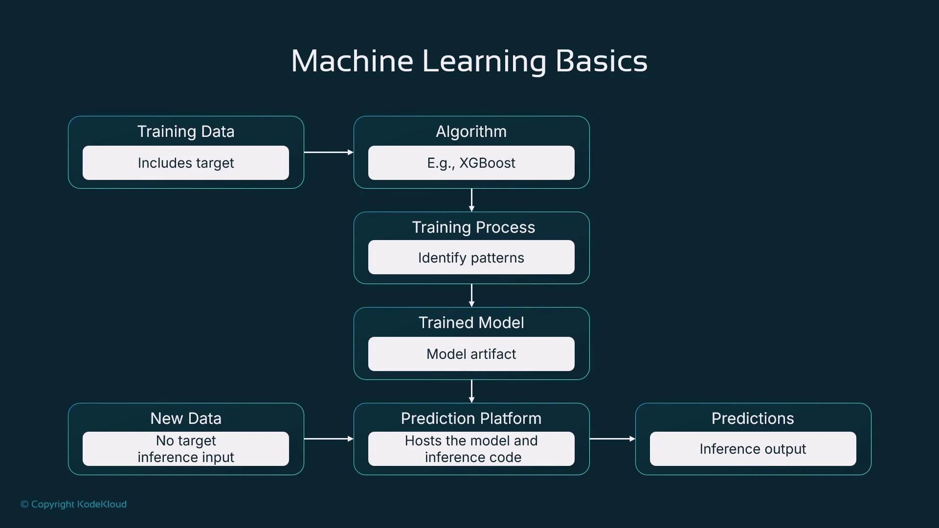
Your training dataset must include the target value for each training example. Supervised learning cannot learn the input→output mapping without that target column.
model.tar.gz or model.tgz) that encodes the learned parameters.
Once training completes, host the model artifact on a prediction platform (a server, virtual machine, or a managed service such as AWS SageMaker). An inference request provides the same input features used in training but omits the target; the model returns a predicted value (for example, “£320,000”).
- Classifying objects (e.g., fraudulent transaction vs. legitimate).
- Forecasting trends (e.g., next-month sales).
- Identifying non-obvious relationships for business intelligence and decision-making.
- We predict house price from a single input feature (for example, property size) to introduce the idea of fitting.
- Plot the (x, y) points (size vs. price). A line that approximates these points is the model: it gives a rule to predict
yfrom a newx.
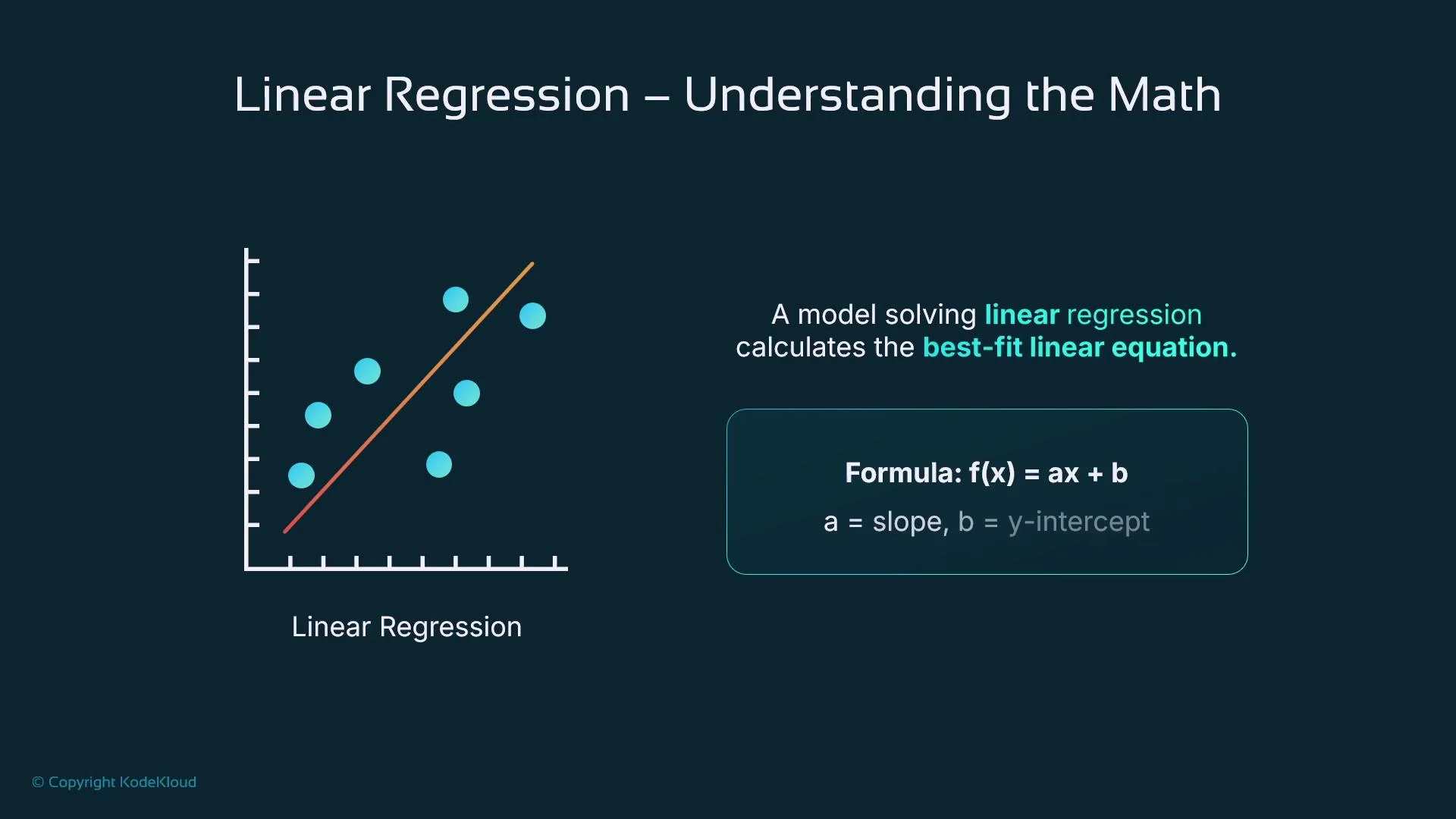
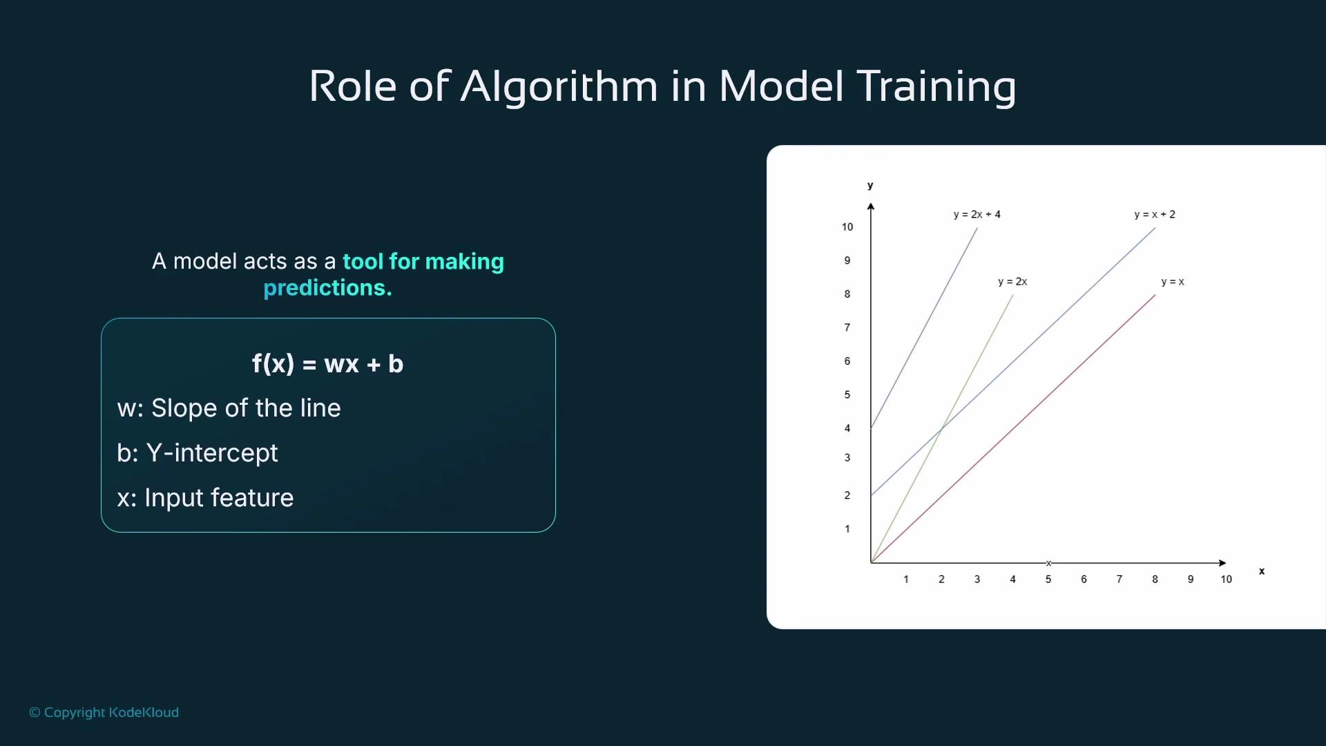
- A line is commonly written as
f(x) = a x + b. In ML we usually writef(x) = w x + bwhere:wis the weight (coefficient) and controls the slope.bis the bias (intercept) and shifts the line vertically.
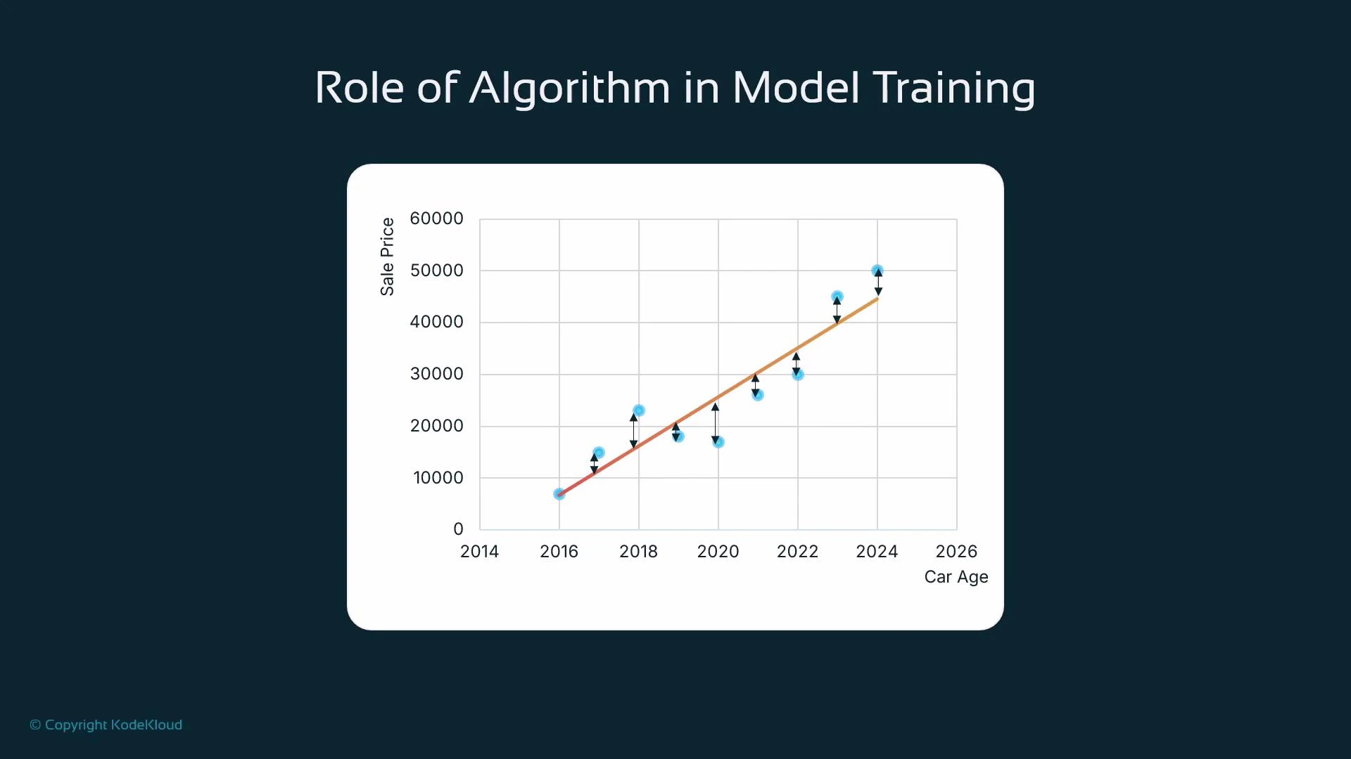
- The line typically does not pass exactly through all points. The vertical distance from an observed point to the line is the residual (error).
w and b to minimize this loss — searching for the line of best fit.
Training is an optimization procedure: the algorithm updates parameters, recomputes the loss, and repeats until it reaches a minimum (local or global).
- With several input features (for example, bedrooms, bathrooms, square footage, age), linear regression generalizes to a weighted sum:
f(x) = w1*x1 + w2*x2 + ... + wn*xn + b
- Each feature
xigets its own weightwi. As the number of features grows (tens to hundreds), the parameter space becomes high-dimensional. - Larger models can capture more complexity but are more prone to overfitting (learning training set noise rather than general patterns). Practical training uses validation data and regularization to manage this trade-off.
| Term | Meaning | Example |
|---|---|---|
Weight (w) | Coefficient applied to a feature | In y = 2x + 4, w = 2 |
Bias (b) | Intercept term, shifts predictions | In y = x + 2, b = 2 |
- Many algorithms use gradient-based optimization (for example, gradient descent) which computes the gradient of the loss with respect to each parameter and updates parameters in the direction that reduces loss.
- The learning rate controls the update step size:
- Too large → risk of overshooting minima and unstable training.
- Too small → slow convergence and high compute cost.
- Stopping criteria: maximum number of iterations/epochs, minimum improvement threshold, or early stopping based on validation loss. These help prevent wasted compute and reduce overfitting.
| Algorithm family | When to use | Typical strengths |
|---|---|---|
| Linear models | Simple relationships, interpretability | Fast, low variance |
| Tree-based (XGBoost, LightGBM) | Tabular data with mixed feature types | High accuracy, handles heterogeneity |
| k-NN | Small datasets, non-parametric | Simple, few assumptions |
| Neural networks | Complex interactions, large datasets | High capacity, requires more data |
Be cautious with many features or overly long training runs: they increase the risk of overfitting and unnecessary compute costs. Use held-out validation data, regularization, and early stopping to monitor generalization.
- Prepare training data: include features and the target column for each example.
- Choose an algorithm suitable for the problem and data modality (tabular, text, images).
- Train iteratively to minimize a loss function (for regression, often sum of squared errors).
- Validate and tune hyperparameters (learning rate, regularization, model complexity).
- Export the trained model artifact and host it on a prediction platform to serve inference requests (new inputs without targets).
- Monitor model performance in production and retrain as needed with new data.
- AWS SageMaker (course)
- XGBoost: https://xgboost.readthedocs.io/
- Scikit-learn (linear models): https://scikit-learn.org/stable/modules/linear_model.html
w and b using Python-style pseudocode.