Multivariate inputs: moving to higher dimensions
Real datasets include many attributes: age, color, sunroof, mileage, alarm, and more. As you add features you move into higher-dimensional input space (five features ⇒ five dimensions). While visualization becomes difficult beyond three dimensions, the mathematics stays the same: the model combines numeric inputs with learned weights to make predictions. To train models, every input must be numeric. Categorical and boolean features must be encoded; continuous features may need scaling. The diagram below illustrates encoding multiple car features before feeding them to a learning algorithm.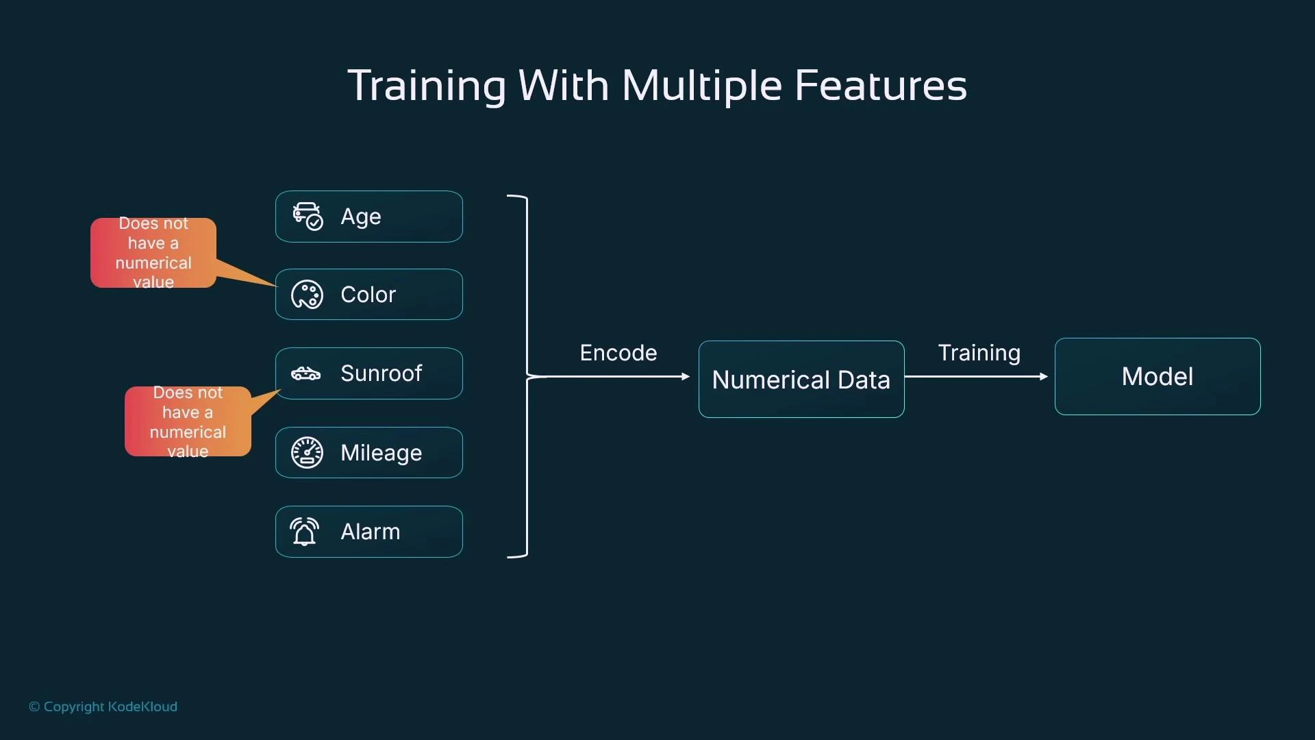
Encoding and preprocessing — best practices
Common encodings and preprocessing choices:| Feature type | Typical encoding | When to use |
|---|---|---|
| Categorical (unordered) | One-hot encoding | Use for nominal categories like color |
| Categorical (ordered) | Label / ordinal encoding | Use only when categories have natural order |
| Boolean | 0 / 1 | Direct binary representation for flags (sunroof, alarm) |
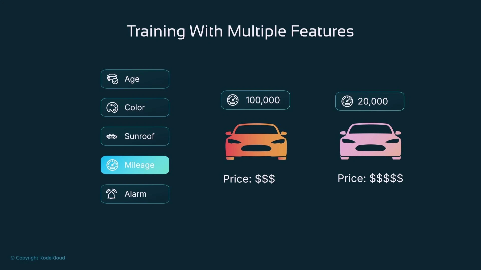
| Numerical | Scaling / normalization (standardize or min-max) | Keep feature magnitudes comparable (e.g., mileage) |
- One-hot is preferred for unordered categories to avoid implying an order.
- Boolean flags map cleanly to 0/1.
- Scale numeric features (e.g., express mileage in thousands or standardize) so learned weights have reasonable magnitudes.
Feature symbols and weights
Assign a symbol to each input feature and a corresponding weight (coefficient) that indicates its influence:- X1 = age
- X2 = color (encoded)
- X3 = sunroof (0/1)
- X4 = mileage
- X5 = alarm (0/1)
Linear model — combining features
A simple linear model predicts a target as a weighted sum of features plus a bias: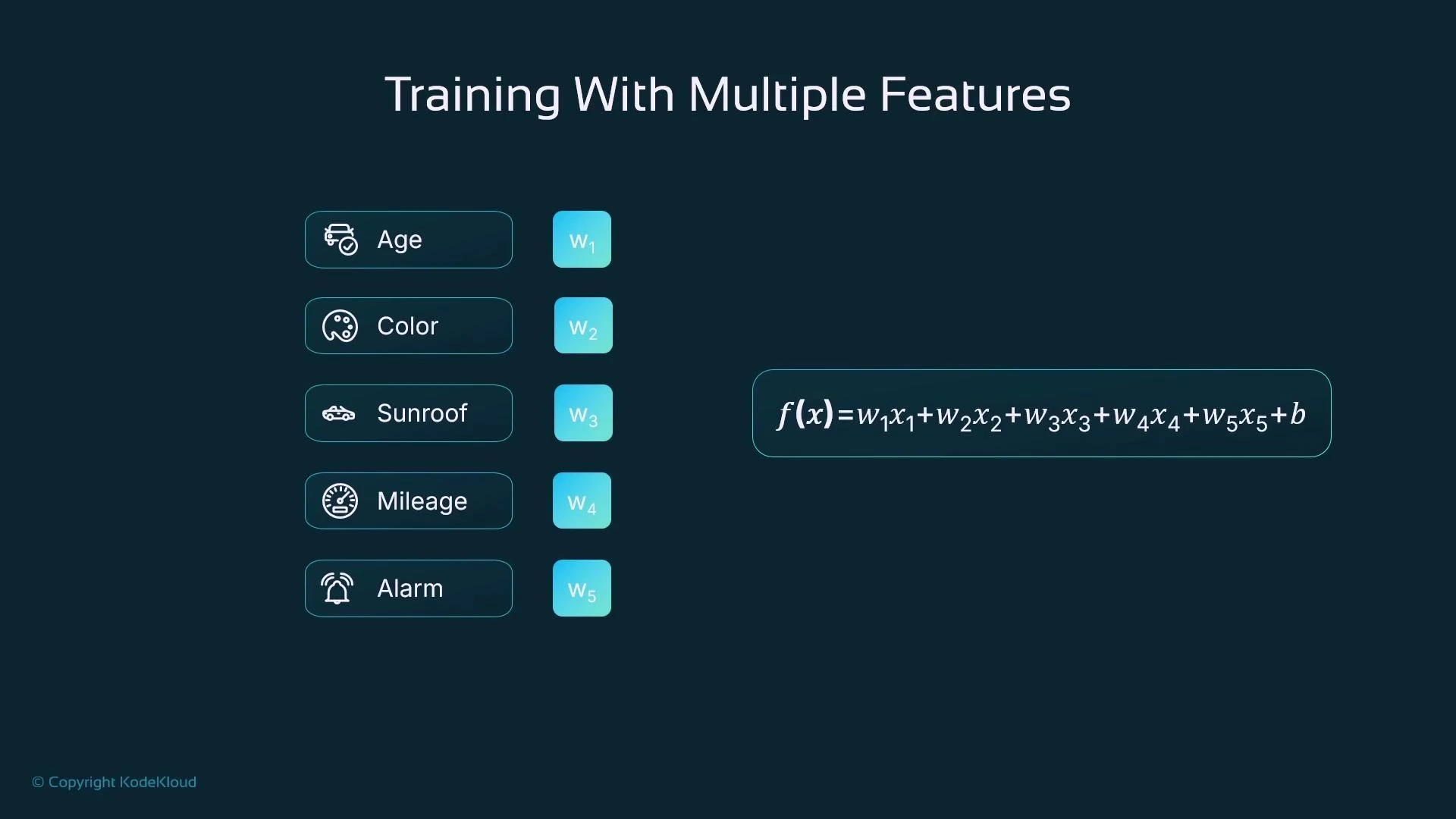
Training objective and loop
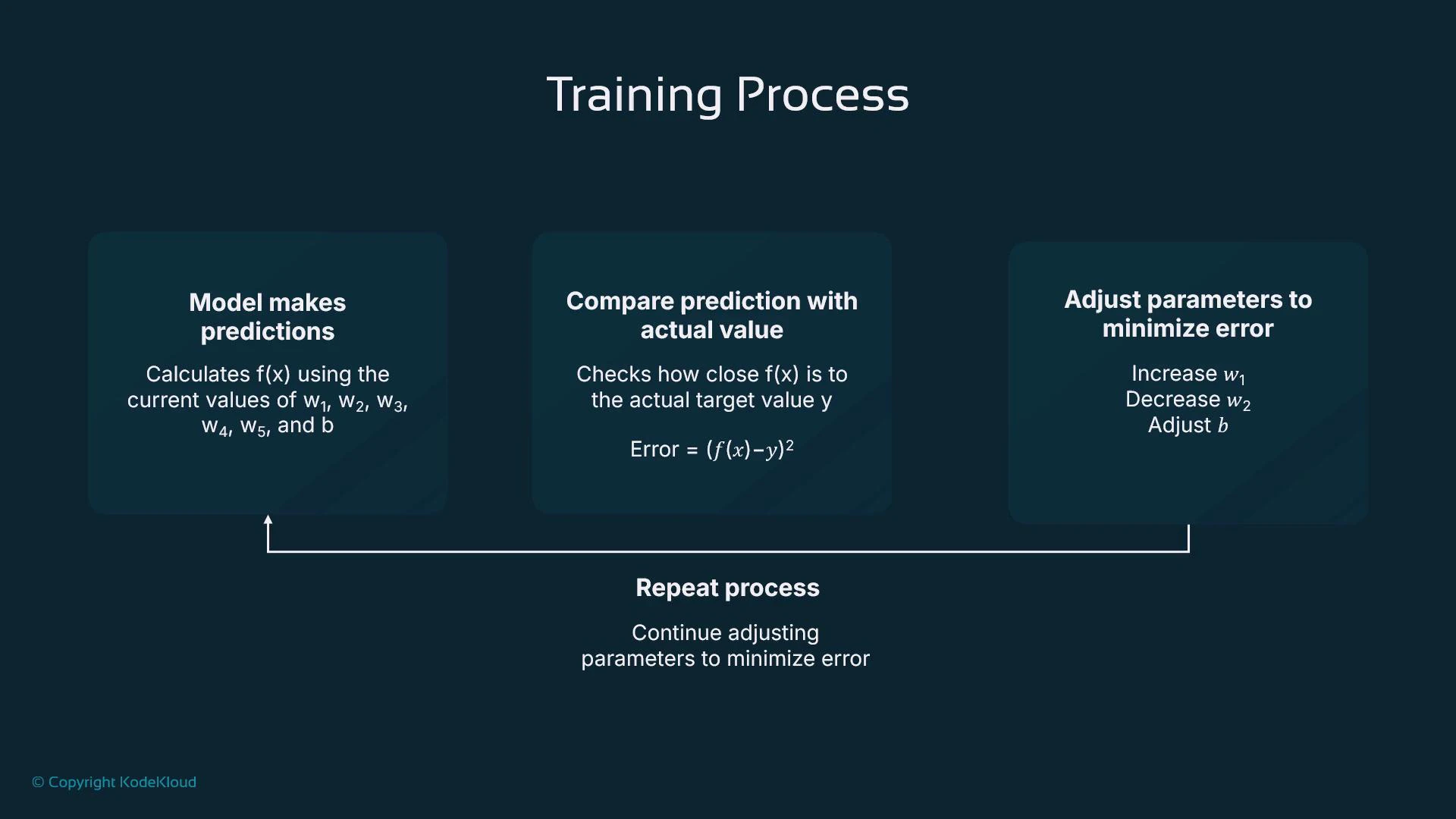
Training optimizes parameters (w1…w5 and b) to minimize a loss function. For regression, the mean squared error (MSE) or sum of squared errors is common. For a single sample:- Initialize parameters (randomly or with sensible defaults).
- Compute predictions f(x) for training samples.
- Compute the loss (how far predictions differ from targets).
- Adjust parameters to reduce the loss (gradient descent or another optimizer).
- Repeat until convergence or another stopping condition.
Numeric example
Here’s an example showing trained parameters and a prediction (mileage scaled to thousands):From training to hosting and inference
Training uses labeled data (inputs with known targets), enabling the model to compare predictions to ground truth and improve. After training, you deploy (host) the trained model on a compute platform (virtual machine, container, on-prem server, or managed service like SageMaker). The hosted model receives new input data (same features, without targets) and returns predictions by applying the learned function f(x).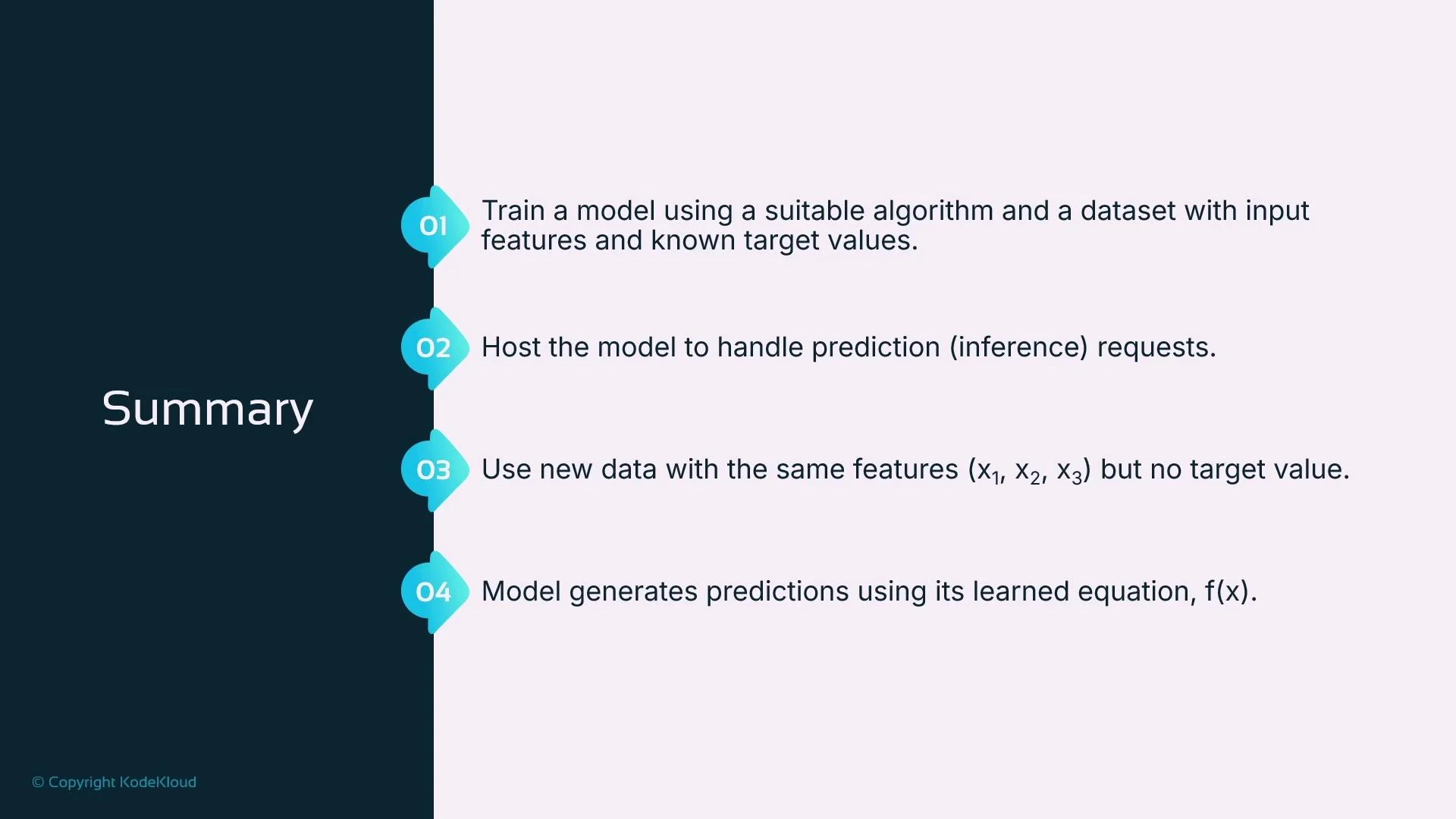
Key takeaways
- ML models learn numeric relationships between features and a target by tuning weights and biases.
- Encode categorical and boolean features numerically before training (prefer one-hot for unordered categories).
- Scale numerical features to keep weights at reasonable magnitudes and improve optimizer behavior.
- Training minimizes a loss function (e.g., squared error) using optimization methods such as gradient descent.
- Ensure the same preprocessing pipeline is applied to training and inference data to avoid serving errors.
Always ensure your training and inference data use the same feature format and preprocessing (encoding and scaling). Mismatches between training and serving preprocessing are a common source of errors.
Further reading and references
- Amazon SageMaker — model training and hosting: https://aws.amazon.com/sagemaker/
- Scikit-learn preprocessing (one-hot, scaling): https://scikit-learn.org/stable/modules/preprocessing.html
- Introduction to Gradient Descent (blog/notes): https://developers.google.com/machine-learning/crash-course/gradient-descent