- Handling missing values (drop vs. impute).
- Removing duplicate rows and redundant columns.
- Enforcing consistency of feature names and data formats.
- Detecting outliers and applying appropriate scaling.
- Sampling strategies for very large datasets.

Consistency checks
Before heavy EDA or modeling, look for inconsistent formatting or naming that will cause bugs or misleading statistics:- Are categorical values consistent? (e.g., “suburban” vs “Suburb” vs “Suburban ”)
- Are date formats uniform (MM/DD/YYYY, DD/MM/YYYY, ISO 8601)?
- Are numeric columns stored as numeric dtypes rather than strings?

Outliers and scaling
Outliers can skew summary statistics (mean, variance) and harm models that rely on gradient or distance calculations. Also watch for features on very different scales — e.g., square footage (hundreds to thousands) vs. number of bedrooms (1–10) — which normally need scaling for many algorithms.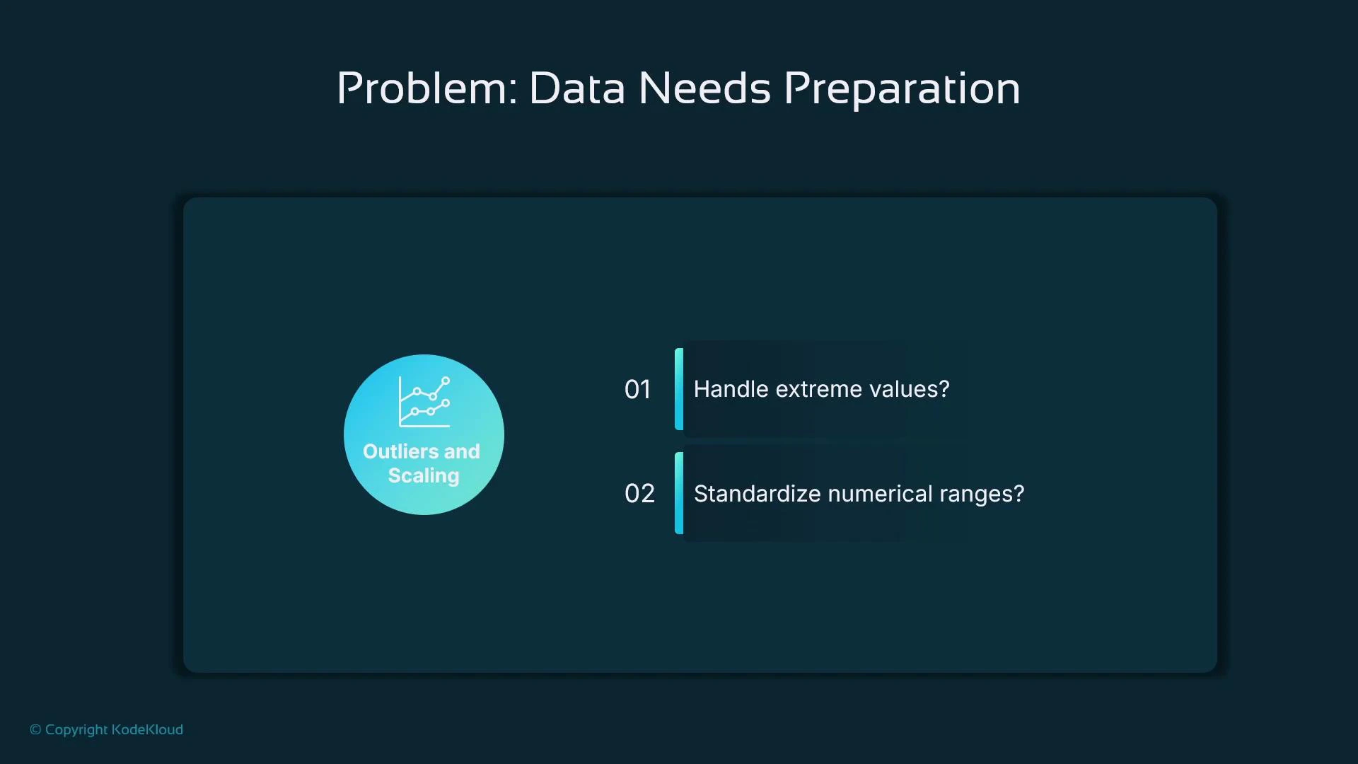
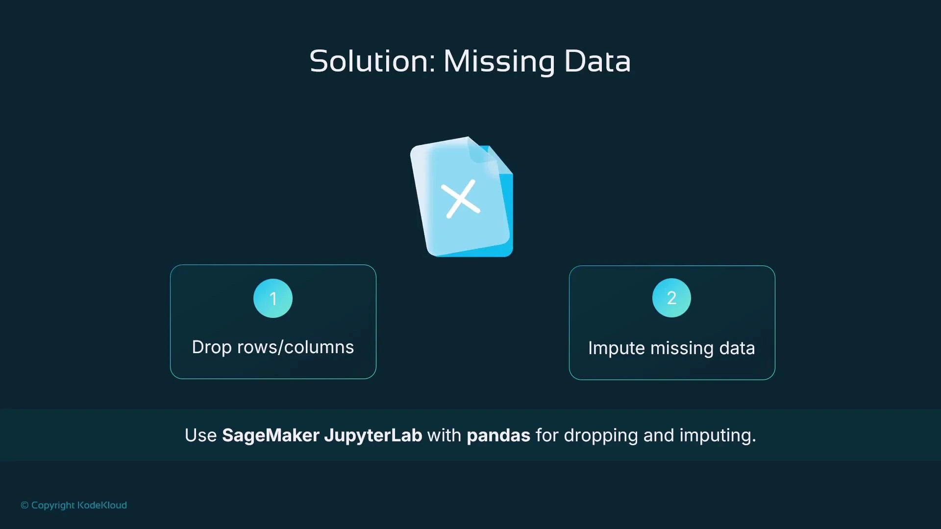
Solution: Missing data
Missing values reduce the model’s ability to learn from the full dataset. Typical choices:- Drop rows or columns with missing values (lossy).
- Impute (fill) missing values with reasonable estimates (preserves rows).
Dropping rows or columns with pandas
Use dropna when you prefer to remove missing data entirely (be mindful of how much data is lost).Imputation with scikit-learn’s SimpleImputer
Imputation preserves dataset size and often helps models when applied sensibly. Choose strategy per feature type:- Numeric: mean, median (robust to outliers), or a constant.
- Categorical: most_frequent (mode) or a special token.
Imputation strategy matters. For skewed numeric features, prefer median over mean. For time-series or grouped data, consider group-wise imputation (e.g., median per region) rather than a global statistic.
Standardizing numeric features
Standardization (zero mean, unit variance) helps gradient-based optimizers converge faster and benefits distance-based algorithms.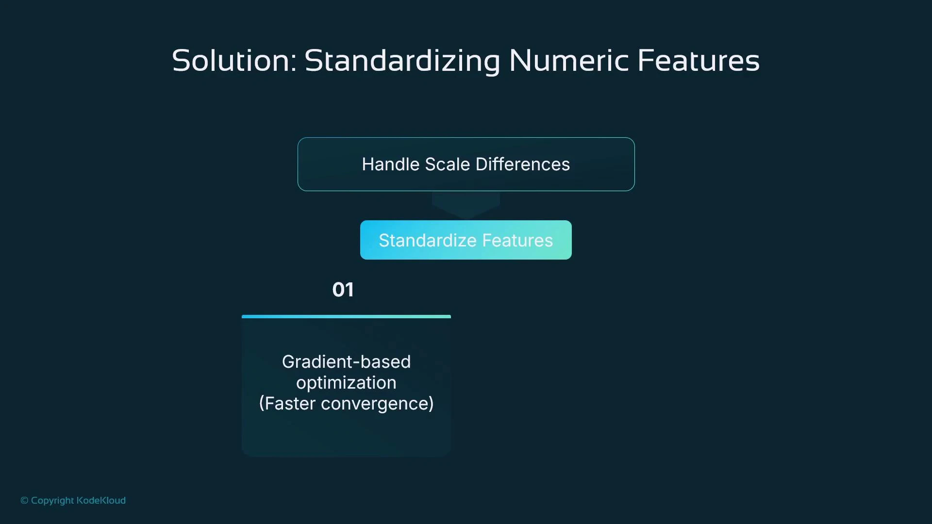
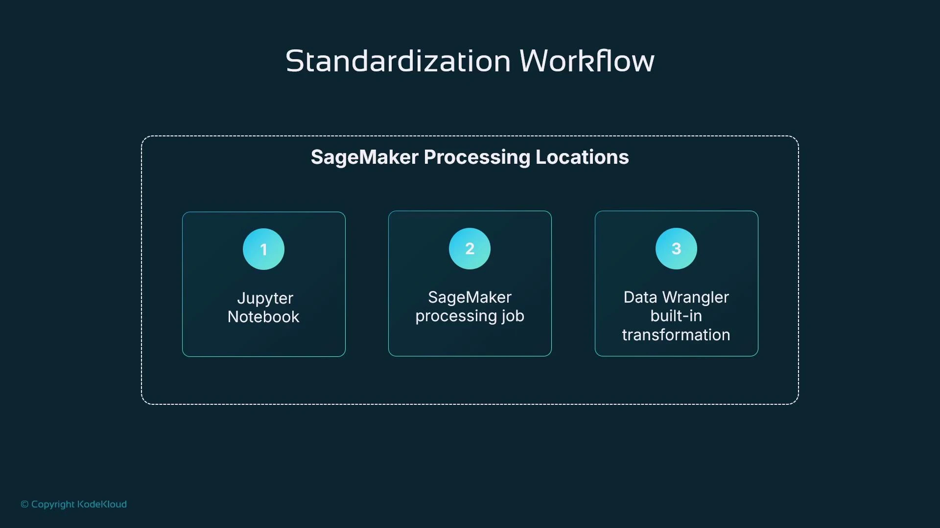
Where to run these transformations
Choose the execution environment based on dataset size and reproducibility requirements.| Resource Type | Use Case | Example |
|---|---|---|
| Local Jupyter | Small exploratory datasets and rapid iteration | Jupyter Notebook / JupyterLab |
| Managed processing | Large datasets or heavy compute, reproducible pipelines | SageMaker Processing |
| Low-code GUI | Users who prefer point-and-click transformation | SageMaker Data Wrangler / SageMaker Canvas |
Categorical data: encoding strategies
Most ML algorithms require numeric inputs, so convert categorical variables to numbers. Choose an encoding based on cardinality and whether categories are ordered.- Ordinal encoding: use when categories have a meaningful order (e.g., low < medium < high).
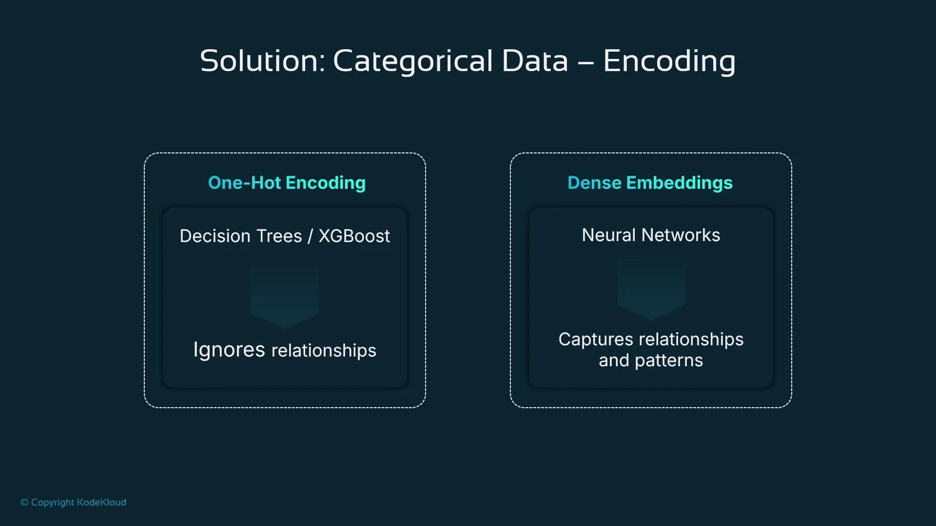
- One-hot encoding: creates binary indicator columns for unordered categories.
- Dense embeddings: learned vector representations for high-cardinality categories (useful with neural nets).
| Encoding Type | Best For | Notes |
|---|---|---|
| Ordinal | Ordered categories | Keeps ordering but assumes uniform gaps |
| One‑hot | Low cardinality, tree-based models | Increases feature width |
| Embeddings | Neural networks; high-cardinality | Compact, captures relationships |
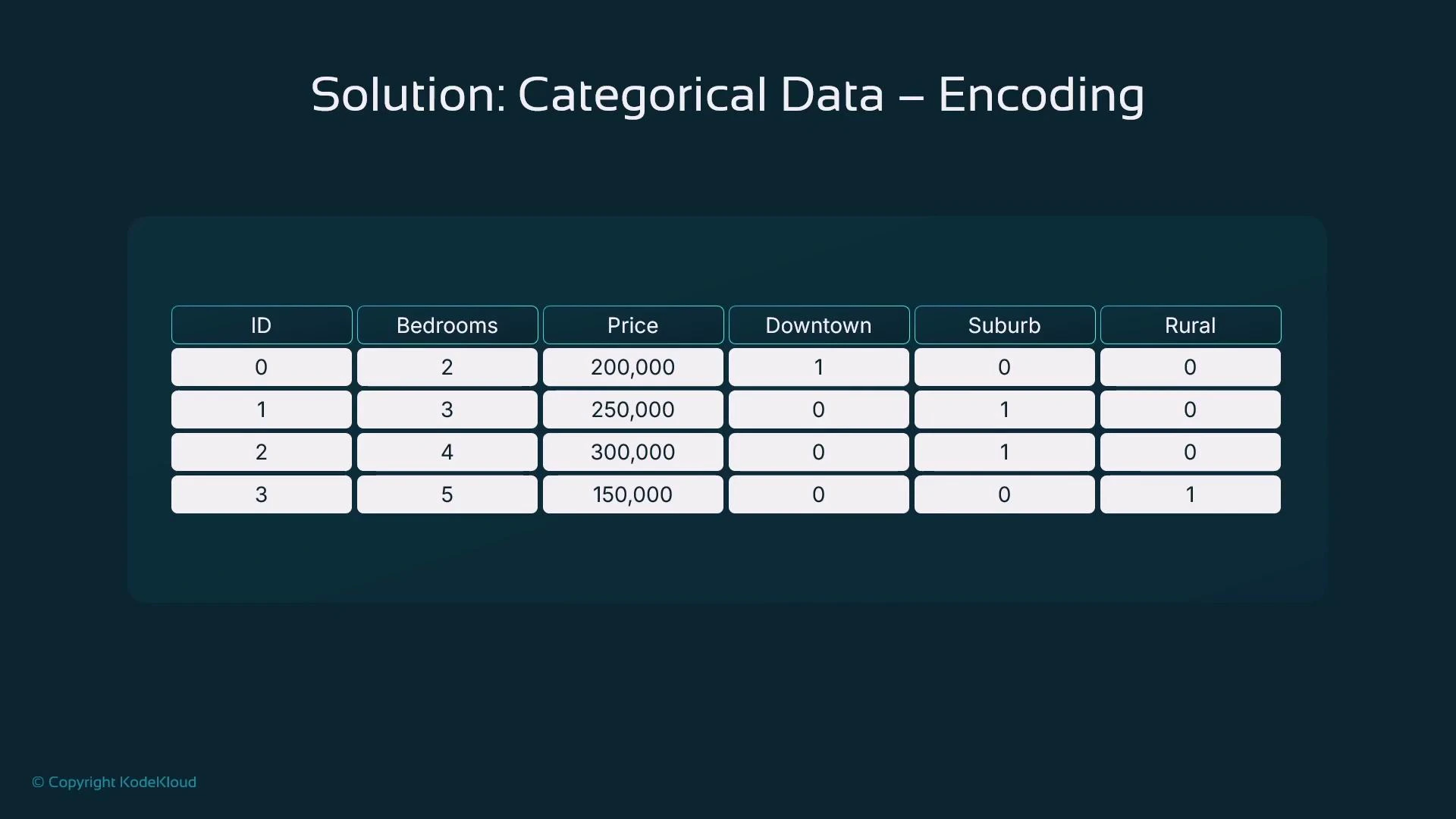
One-hot encoding example with pandas.get_dummies
Use drop_first=True when you need to avoid perfect multicollinearity for linear models.Handling outliers
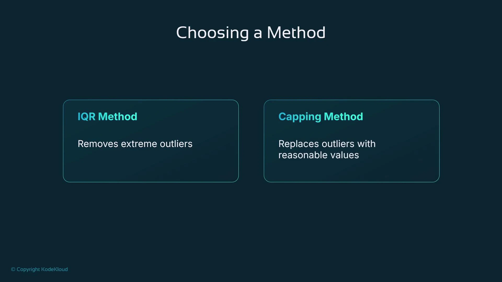
Choose an approach depending on whether you need to preserve rows:- IQR filtering — removes extreme outliers (row loss).
- Percentile capping (winsorization) — replaces outliers with percentile boundaries (no row loss).
IQR filtering example
Percentile capping (clip) example
Do not remove outliers blindly. Investigate whether extreme values are data errors, rare-but-valid cases, or important signals (e.g., luxury properties). Choose removal or capping based on domain context and downstream model sensitivity.
- IQR filtering removes extreme values (reduces dataset size).
- Capping replaces extreme values with boundary values (keeps row count).
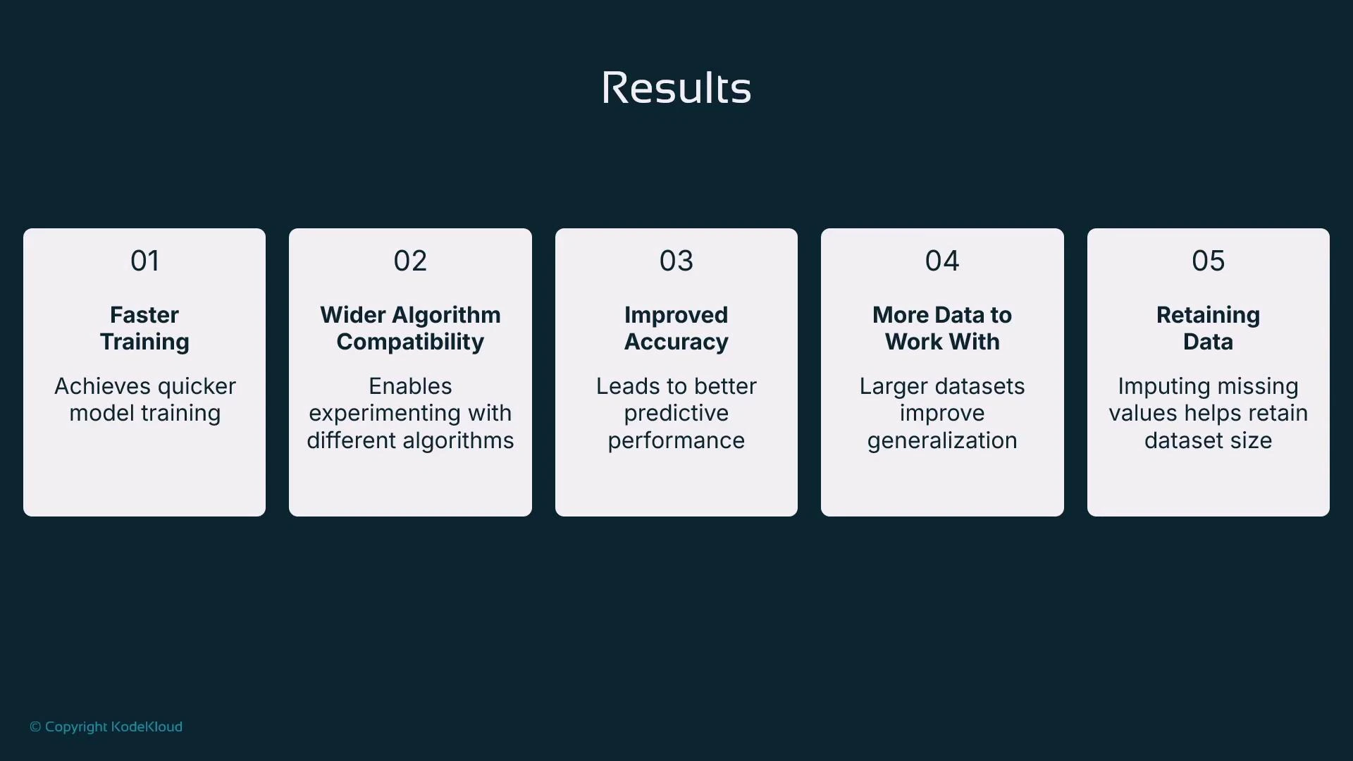
Results you can expect from good preparation
- Faster and more stable training (models can identify relationships more easily).
- Greater algorithm flexibility (prepared data works across SVMs, KNN, XGBoost, neural nets).
- Better generalization and predictive performance.
- Ability to retain more data via imputation rather than dropping records.
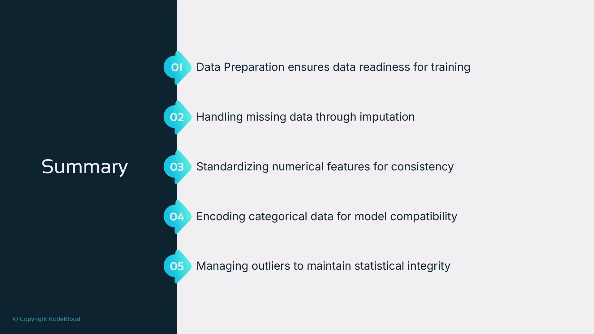
Summary
- Preparing tabular data substantially improves readiness for training and typically results in faster convergence and better model quality.
- Use imputation methods (mean, median, mode) to retain dataset size when sensible.
- Standardization (StandardScaler) prevents large-scale features from dominating learning.
- Convert categorical variables using one-hot, ordinal, or embeddings depending on model type and cardinality.
- Handle outliers with IQR filtering or percentile capping depending on whether you want to remove or preserve rows.
- pandas Documentation
- scikit-learn Documentation
- Jupyter Project
- Amazon SageMaker Processing
- SageMaker Data Wrangler
- SageMaker Canvas