A pragmatic path: learn the math you need for practical steps today (data cleaning, encoding, scaling, evaluation). Deeper math (linear algebra, probability, optimization) is valuable later for advanced model design and research.
Two realistic learning paths
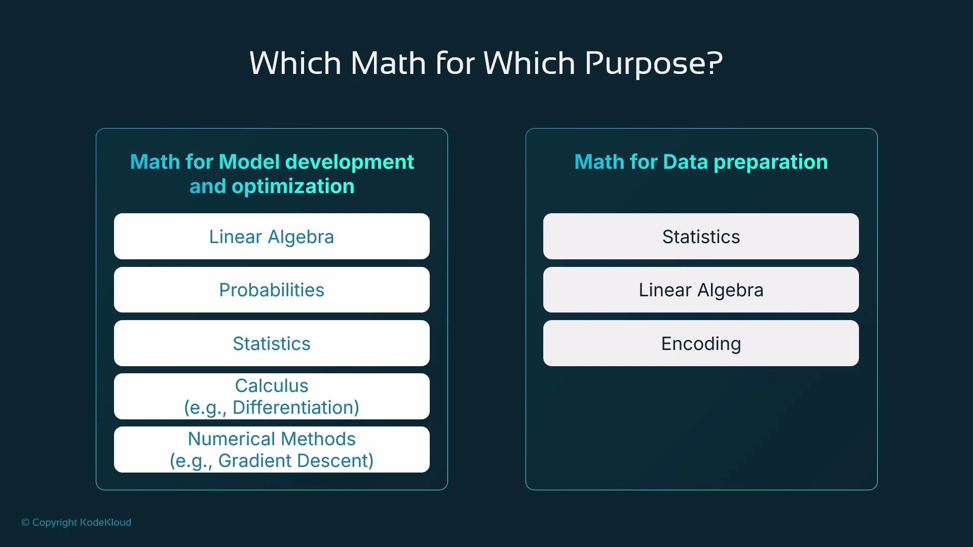
Which path you choose depends on your role and goals. Below is a concise comparison.| Role | Required math focus | Typical tasks |
|---|---|---|
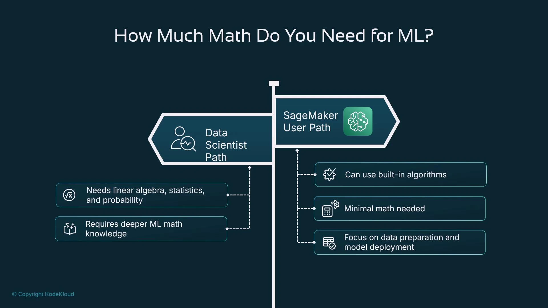
| Data Scientist | Linear algebra, probability, statistics, calculus, numerical optimization | Build and customize models, tune hyperparameters, design new algorithms |
| SageMaker / ML Practitioner | Basic statistics, encoding techniques, data preparation, model evaluation | Prepare datasets, use built-in algorithms, integrate models into applications, deploy and monitor |
What happens during training (intuitively)
For tabular data, many models express predictions as functions of weighted inputs. A simple linear-style model looks like: f(x) = w1x1 + w2x2 + w3*x3 + … + b Training adjusts the weights (w1, w2, …) and bias b to make predictions f(x) close to known target values. The model uses a loss function (e.g., mean squared error) to quantify prediction error and applies numerical optimization (such as gradient descent) to reduce that loss iteratively.
Focus: data preparation techniques that matter most
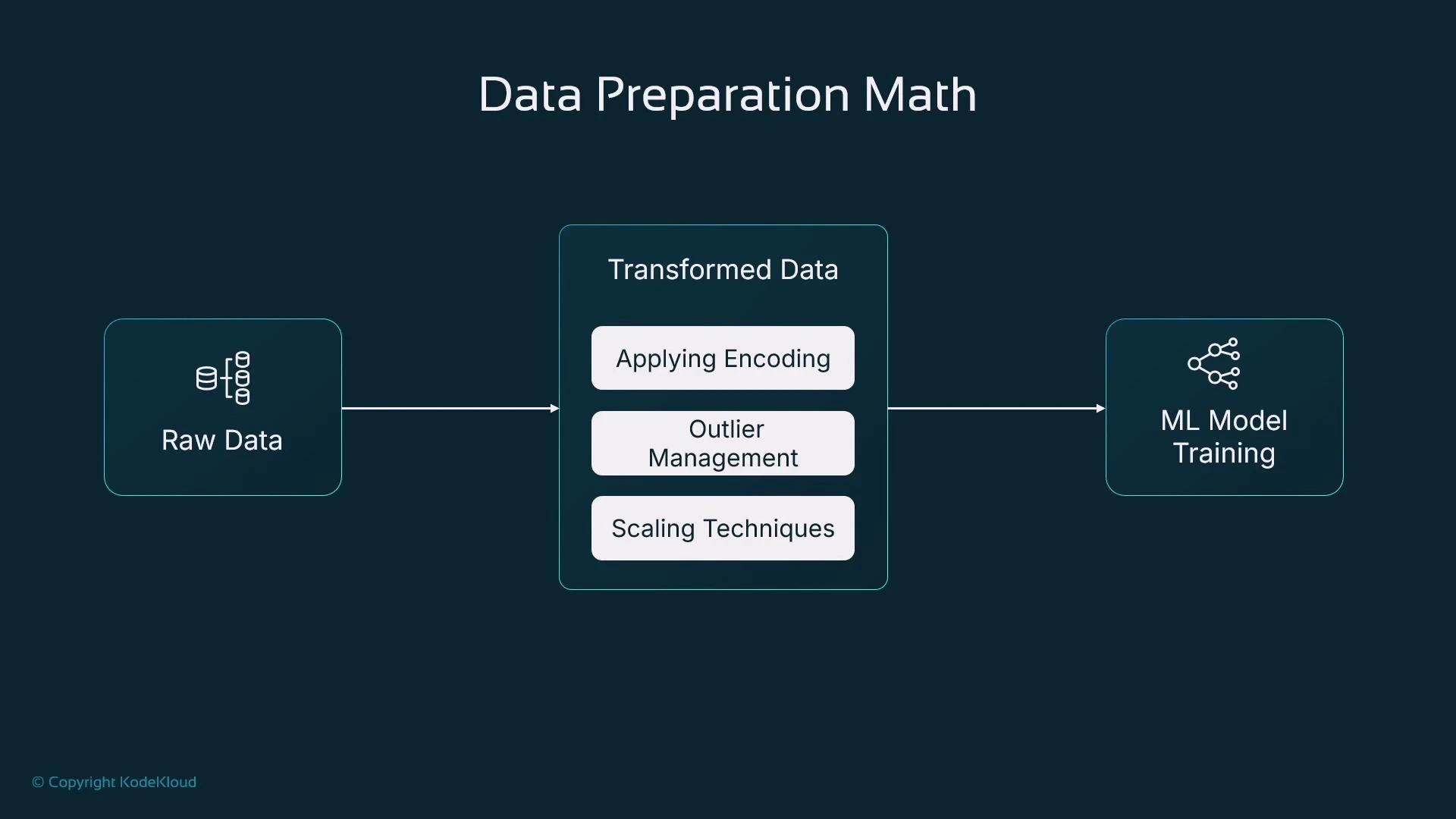
For most practical ML tasks, applying a small set of preprocessing techniques will yield large improvements in model performance. Key techniques:- Encoding: convert categorical variables into numeric representations (one-hot, ordinal, target encoding).
- Outlier management: detect and handle extreme values (capping, clipping, transforms, or robust methods).
- Feature scaling: standardization, min-max scaling, or robust scaling depending on algorithm sensitivity.
Python tools commonly used
Pandas and scikit-learn are the standard libraries for preprocessing and basic modeling.Outliers: detection and handling
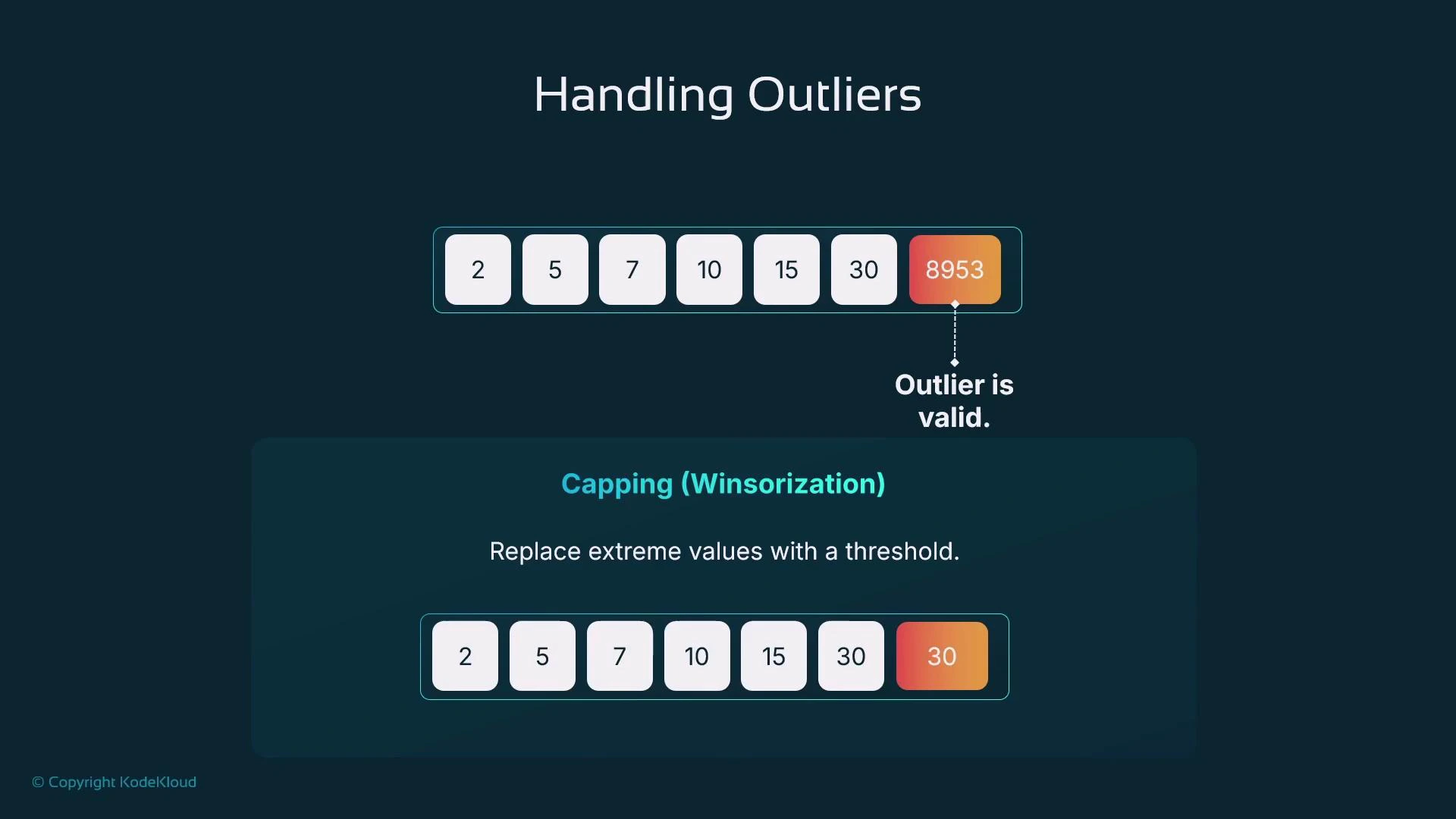
An outlier is a value that deviates significantly from the rest of a distribution. Outliers can distort summary statistics such as the mean. For example: 2, 5, 7, 10, 15, 30, 8953 Including 8953 makes the mean ~1288.9 (misleading); excluding it yields a mean of 11.5 for the remaining values. Deleting data outright is not always appropriate—consider the cause and the downstream impact before removing values.![A slide titled "Handling Outliers" showing the dataset [2, 5, 7, 10, 15, 30, 8953] with 8953 highlighted as an extreme outlier. It illustrates that including the outlier produces a misleading mean (~1288) while excluding it gives a more representative mean (11.5).](https://mintcdn.com/kodekloud-c4ac6d9a/VCFuPHSNLDaVdMaA/images/AWS-SageMaker/Machine-Learning-Prerequisites/How-Much-Math-Do-I-Need/handling-outliers-8953-inflated-mean.jpg?fit=max&auto=format&n=VCFuPHSNLDaVdMaA&q=85&s=a0dd3d38be0dba89665c5c9f94ecbb69)
- Was it a data-entry error or a pipeline corruption? If so, correct or remove it.
- If the value is valid but extreme, choose a strategy: capping (Winsorization), clipping, transformation (log, sqrt), or use robust methods (robust scalers, median-based statistics).
IQR method (practical outlier detector)
The Interquartile Range (IQR) method is robust and easy to implement. IQR steps:- Sort data.
- Q2 = median (50th percentile).
- Q1 = median of the lower half (25th percentile).
- Q3 = median of the upper half (75th percentile).
- IQR = Q3 − Q1.
- Outlier bounds: [Q1 − 1.5IQR, Q3 + 1.5IQR].
- Sorted: [2, 5, 7, 10, 15, 30, 90]
- Q1 = 5, Q2 = 10, Q3 = 30 → IQR = 25
- Bounds: [-32.5, 67.5] → 90 is an outlier.
![A slide illustrating how to compute the interquartile range (IQR) from the dataset [2, 5, 7, 10, 15, 30, 90]. It shows Q1=5, Q2=10, Q3=30, IQR=25, bounds -32.5 and 67.5, and flags 90 as an outlier.](https://mintcdn.com/kodekloud-c4ac6d9a/o0DMf8IaEQ0yghSZ/images/AWS-SageMaker/Machine-Learning-Prerequisites/How-Much-Math-Do-I-Need/iqr-calculation-outlier-90-slide.jpg?fit=max&auto=format&n=o0DMf8IaEQ0yghSZ&q=85&s=7584e06112ec0781f31cbdfb0242e5a2)
- Computes Q1 and Q3 using pandas quantile.
- Determines thresholds using the 1.5*IQR rule.
- Uses np.clip to cap values to those thresholds (Winsorize).
- Remove outliers if they are errors.
- Apply log or other transforms to reduce skew.
- Use RobustScaler in scikit-learn, which uses median and IQR for scaling.
Be careful removing data solely to improve model metrics. Validate outliers against domain knowledge—rare but correct observations may be important signals.
Feature scaling: when and how
Feature scaling makes numeric features comparable. Algorithms that rely on distances (k-NN, clustering) or gradient updates (logistic regression, neural networks) benefit most. Common scalers:- StandardScaler: subtract mean, divide by standard deviation → zero mean, unit variance.
- MinMaxScaler: scale to [0, 1] (or another fixed range).
- RobustScaler: subtract median, scale by IQR → less sensitive to outliers.
- Use RobustScaler when outliers are present and you want robustness.
- Use StandardScaler for algorithms that assume Gaussian-like data or need standardized inputs.
- Use MinMaxScaler for bounded inputs (e.g., image pixel normalization to [0,1]).
Summary: what to prioritize
You do not need to master all mathematics before starting ML. Prioritize practical skills that improve model performance quickly:- Basic statistics and exploratory data analysis (EDA)
- Handling missing values and outliers
- Encoding categorical variables correctly
- Applying appropriate scaling to numeric features