Feature engineering is the process of transforming prepared dataset columns into representations that are more useful for a chosen machine learning algorithm. It sits between dataset preparation (cleaning, imputation) and model training. Good feature engineering can improve predictive performance, reduce training time, and make models more robust.
A dark-blue presentation slide from KodeKloud. The title reads "Feature Engineering – Introduction" with the subtitle "Theory" and the KodeKloud logo at the top.
We will show practical examples using pandas and scikit-learn and demonstrate how to scale these transformations using SageMaker Processing jobs. Typical feature-engineering tasks include encoding categorical variables, selecting or creating features, transforming skewed data, aggregating information, and scaling numeric inputs.
A presentation slide titled "Agenda" listing four items: Problem (prepared data may not be enough), Solution (apply feature engineering), Workflow (using Pandas, sklearn, and SageMaker Processing Jobs), and Results (better model performance and faster training). The design shows numbered blue markers down the left with the agenda text on a light background.

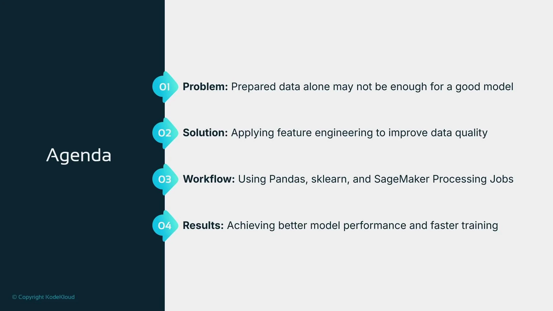
Why feature engineering matters

Even after basic cleaning (e.g., filling missing values), raw data often needs further transformation:
  • Irrelevant or redundant features slow training and may reduce model quality.
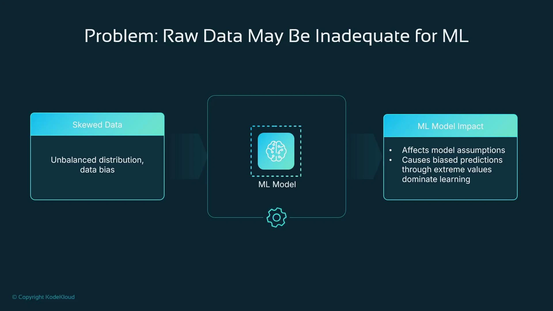
  • Noise or outliers can bias learning and harm generalization.
  • Categorical features must be encoded in ways that reflect their semantics (ordinal vs nominal). Poor choices can mislead models.
  • Strongly skewed numeric inputs can violate algorithmic assumptions and reduce performance.
A presentation slide titled "Problem: Raw Data May Be Inadequate for ML" showing skewed data (unbalanced distribution, data bias) feeding an ML model. The right panel lists ML model impacts like affected assumptions and biased predictions.

Common feature-engineering activities

ActivityPurposeTypical methods / tools
Feature selectionRemove irrelevant or redundant inputs to speed training and avoid overfittingCorrelation analysis, feature importance, recursive feature elimination
Categorical encodingRepresent categorical data numericallyOne-hot, ordinal, target encoding, hashing, embeddings
Feature extractionCreate informative features from raw valuesDate parts, text lengths, tokenization, embeddings
Feature transformationReduce skew and stabilize variancelog, sqrt, power transforms, Box-Cox
Feature interactionsCapture multiplicative or composite effectsMultiplication, concatenation, polynomial features
Aggregation / groupingAdd group-level statisticsgroupby / pivot_table (mean, sum, count)
Scaling / normalizationPut features on comparable scalesStandardScaler, MinMaxScaler
When features have very high cardinality (for example, postal codes or item IDs), prefer techniques that limit dimensionality (target encoding, hashing, or learned embeddings) instead of naive one-hot encoding, which explodes feature count.

Hands-on examples (pandas + scikit-learn)

Start by loading a small sample dataset into a pandas DataFrame for local experimentation:
import pandas as pd
import numpy as np
from sklearn.preprocessing import OneHotEncoder, MinMaxScaler, StandardScaler
from sklearn.model_selection import train_test_split

# Sample dataset
data = {
    "house_size": [1500, 1800, 1200, np.nan, 2000],
    "num_bedrooms": [3, 4, 2, 3, np.nan],
    "city": ["New York", "San Francisco", "New York", "Chicago", "San Francisco"],
    "year_built": [2000, 1995, 2010, 2005, 1998],
    "price": [500000, 700000, 350000, 450000, 750000]
}

df = pd.DataFrame(data)
print("Original Data:\n", df)

Encoding categorical variables

  • One-hot encoding expands nominal categories into binary columns (useful for low-cardinality categorical variables).
  • Ordinal encoding maps categories to integers when a natural order exists.
  • For dates, extract year/month/dayofweek with dt accessor.
  • For text, use length, token counts, or embeddings depending on needs.
# One-hot encoding a nominal column
df_onehot = pd.get_dummies(df, columns=["city"], prefix="city")
print(df_onehot.head())

# Ordinal/label encoding (only when category order is meaningful)
df["city_label"] = df["city"].astype("category").cat.codes
print(df[["city", "city_label"]].head())

# Date example (if you had a 'sale_date' column)
# df['sale_date'] = pd.to_datetime(df['sale_date'])
# df['sale_year'] = df['sale_date'].dt.year
# Text feature example (if you had 'description')
# df['description_length'] = df['description'].str.len()
Be careful with target encoding: if you encode categories using information from the target without proper cross-validation or out-of-fold strategies, you can leak label information and inflate evaluation metrics.

Feature transformations and interactions

  • Use log or sqrt transforms to reduce skew and moderate the influence of extreme values.
  • Create interaction features to capture multiplicative or combined effects.
# Log transform price to reduce skew (use log1p to handle zero safely)
df['log_price'] = np.log1p(df['price'])

# Square root transform (example on house_size)
df['sqrt_house_size'] = np.sqrt(df['house_size'])

# Interaction feature: house size multiplied by number of bedrooms
df['size_bed_interaction'] = df['house_size'] * df['num_bedrooms']

Aggregations and grouping

Group-level statistics can be powerful features (e.g., mean price by city). Use groupby or pivot_table and merge results back into the main DataFrame.
# Group by city and compute mean price
city_price_mean = (
    df.groupby('city')
      .agg({'price': 'mean'})
      .rename(columns={'price': 'mean_price_by_city'})
      .reset_index()
)

# Merge the aggregated feature back into df
df = df.merge(city_price_mean, on='city', how='left')
print(df[['city', 'mean_price_by_city']])

Derived features, missing-value handling, dropping redundant columns, and scaling

Create derived features such as age, handle missing values with imputation strategies, drop original columns if redundant, compute ratios like price per square foot, and scale numeric columns for algorithms that require normalized inputs.
from sklearn.preprocessing import StandardScaler

# Derive house age
df["house_age"] = 2024 - df["year_built"]
print("\nAfter Adding House Age Feature:\n", df[["year_built", "house_age"]])

# Handle missing values by imputing with the median
df["house_size"].fillna(df["house_size"].median(), inplace=True)
df["num_bedrooms"].fillna(df["num_bedrooms"].median(), inplace=True)

# Drop redundant original column if we keep 'house_age'
df.drop(columns=["year_built"], inplace=True)

# Create price per square foot
df["price_per_sqft"] = df["price"] / df["house_size"]

# Standardize a numeric column (zero mean, unit variance)
scaler_standard = StandardScaler()
df["house_size_standardized"] = scaler_standard.fit_transform(df[["house_size"]])

print("\nFinal DataFrame:\n", df.head())

Where to execute feature-engineering code at scale

  • Local development: pandas + scikit-learn on a developer laptop is ideal for prototyping and experiments.
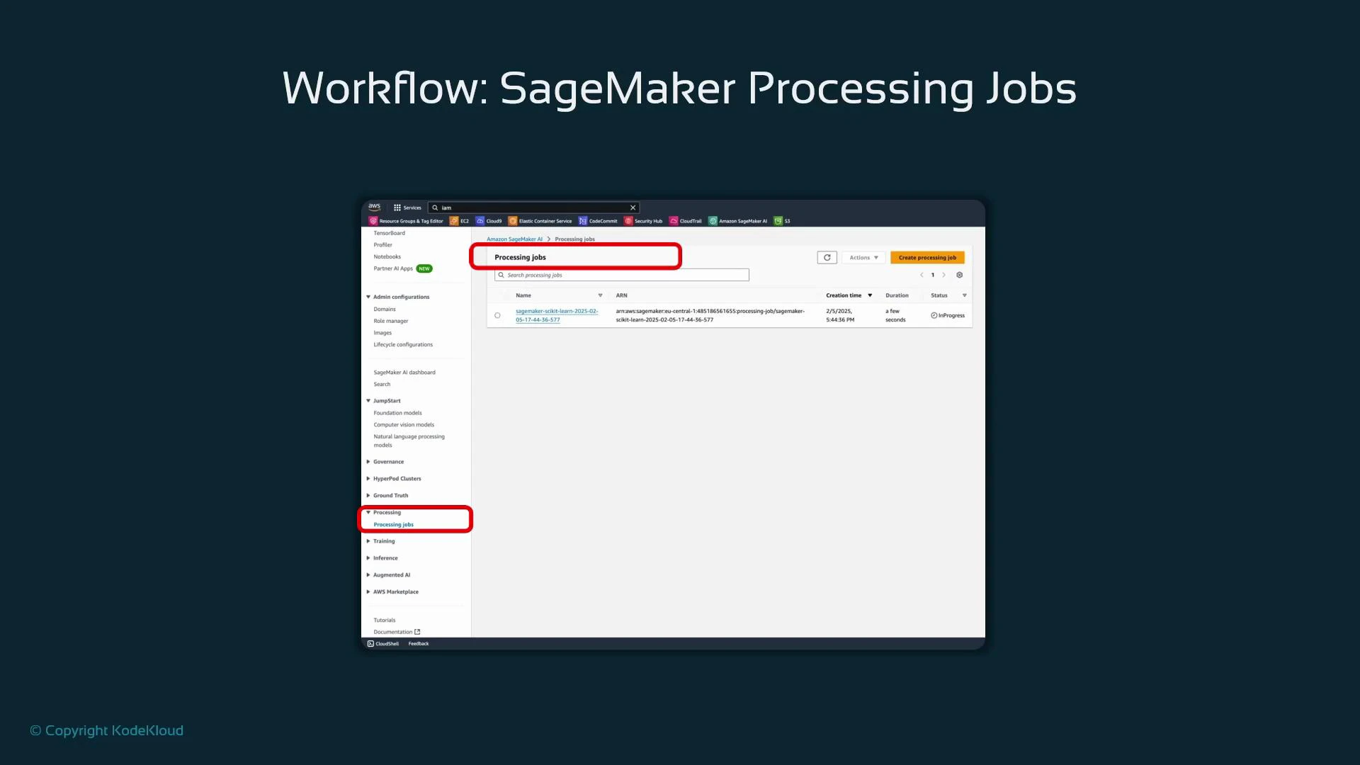
  • Production-scale or repeatable pipelines: use managed compute and orchestration. SageMaker Processing is a common choice to run these transformations on managed instances and produce reproducible outputs.
SageMaker Processing jobs require:
  • A container (framework image, e.g., scikit-learn)
  • A processing script that reads inputs, transforms data, and writes outputs
  • Instance type and count
  • IAM role with appropriate permissions
Example: launch a scikit-learn-based SageMaker Processing job with the SageMaker SDK:
from sagemaker.sklearn import SKLearnProcessor
from sagemaker.processing import ProcessingInput, ProcessingOutput

# Replace with an appropriate IAM role for SageMaker
sagemaker_role = "arn:aws:iam::123456789012:role/SageMakerExecutionRole"

sklearn_processor = SKLearnProcessor(
    framework_version="1.2-1",    # scikit-learn container version
    role=sagemaker_role,
    instance_type="ml.m5.large",
    instance_count=1,
    base_job_name="feature-engineering-job"
)

# Run a processing job that executes 'preprocessing.py' in the provided source directory
sklearn_processor.run(
    code="preprocessing.py",  # your preprocessing script that reads input, transforms, writes output
    source_dir="src",         # directory containing preprocessing.py and dependencies
    inputs=[
        ProcessingInput(source="s3://your-bucket/input-data/", destination="/opt/ml/processing/input")
    ],
    outputs=[
        ProcessingOutput(source="/opt/ml/processing/output", destination="s3://your-bucket/output-data/")
    ],
    wait=True
)
ParameterPurposeExample
framework_versionVersion of the SageMaker scikit-learn container”1.2-1”
instance_typeCompute instance for processing”ml.m5.large”
instance_countNumber of instances to run in parallel1 or more
code / source_dirScript and code dependenciespreprocessing.py in src/
inputs / outputsS3 or local paths for input and output artifactsS3 paths for raw and transformed data
The SageMaker Processing console provides monitoring and logs for jobs and is useful for debugging and auditing runs.
A screenshot of the AWS SageMaker console titled "Workflow: SageMaker Processing Jobs," showing the Processing jobs page with one job listed. The sidebar item and the page header "Processing jobs" are highlighted in red.

Summary and best practices

  • Feature engineering is essential to present the most informative inputs to a model and usually improves performance and convergence speed.
  • Choose encodings and transformations intentionally—consider domain knowledge, algorithm assumptions, and feature cardinality.
  • Prototype locally with pandas and scikit-learn; scale production jobs with SageMaker Processing or other managed services.
  • Always validate feature changes with proper cross-validation and monitor for data leakage (especially with target-based encodings).

Watch Video