

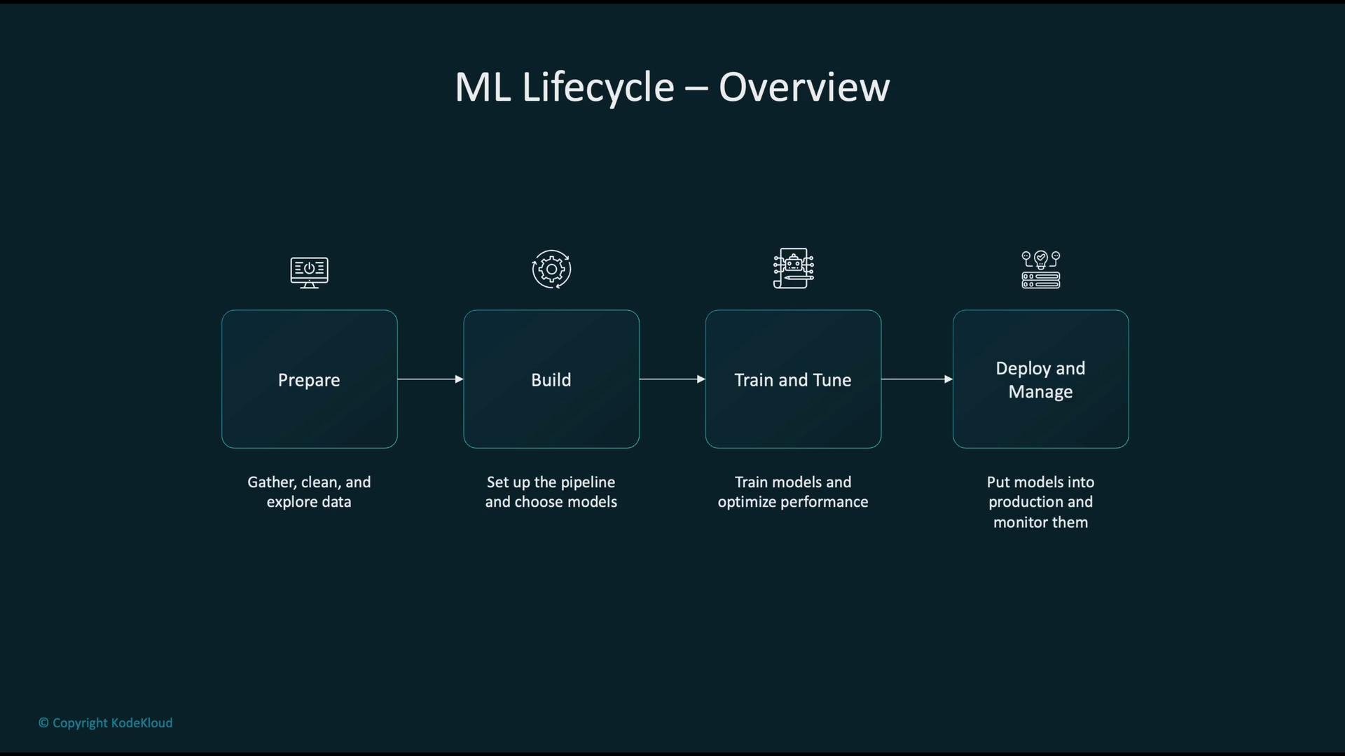
- Prepare: gather, clean, and explore raw data.
- Build: design data pipelines and select appropriate model families.
- Train and Tune: optimize model parameters and hyperparameters.
- Deploy and Manage: release models into production and monitor them continuously.
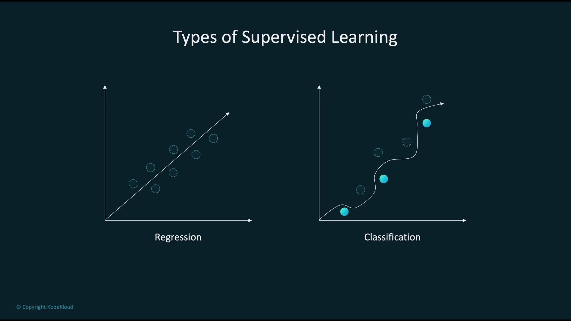
- Regression — predicts continuous values (for example, estimating a house price). Often visualized as fitting a best-fit line or curve to data points.
- Classification — predicts discrete labels (for example, detecting whether an email is spam). Conceptually this finds decision boundaries that separate classes.
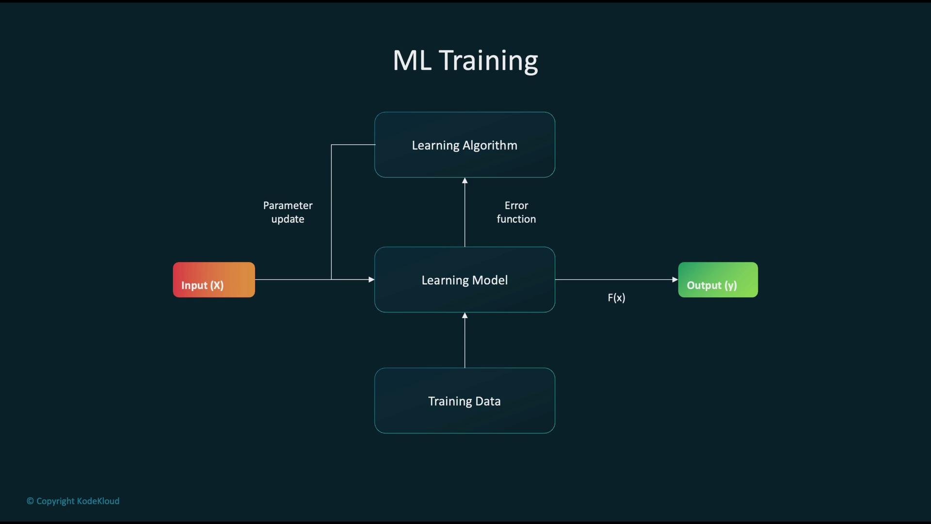
- Feed inputs and training data into the learning model.
- The model produces predictions (outputs).
- Compute an error (loss) using a chosen loss function.
- Pass the error to the learning algorithm (optimizer).
- Update model parameters to reduce error and repeat until convergence.
- Amazon Translate — real-time language translation
- Amazon Rekognition — image and video analysis (objects, faces, content)
- Amazon Transcribe — speech-to-text transcription
- Amazon Polly — text-to-speech synthesis
- Start with a pre-trained base model that encodes general knowledge.
- Add task-specific layers or adapt existing layers for your objective.
- Train on domain-specific data (often with lower learning rates and regularization).
- Validate and iterate until the model meets performance and safety criteria.
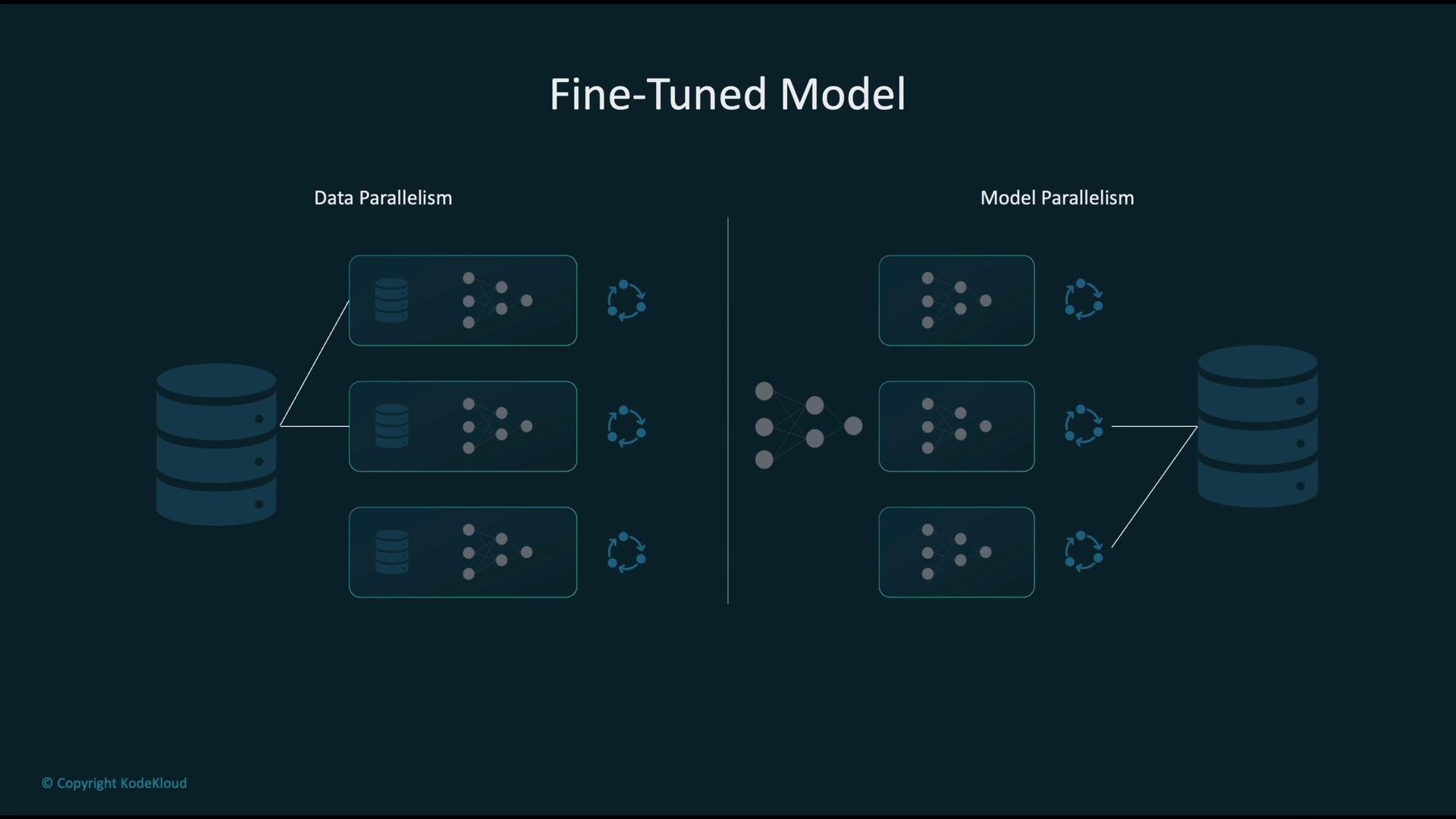
- Data parallelism: replicate the full model across devices; each replica processes a different batch and synchronizes gradients.
- Model parallelism: split the model across devices so a single example flows through model partitions (useful for very large architectures).
- Combine multiple models (averaging, majority voting, stacking).
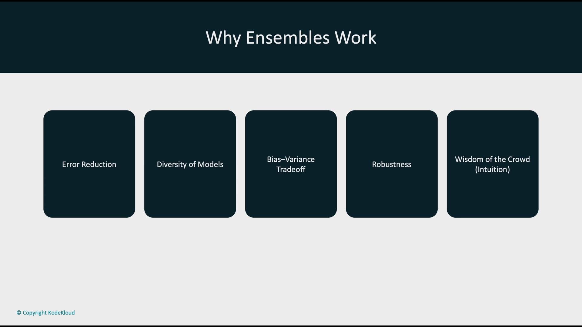
- Benefit from error reduction: different models make different errors.
- Help manage the bias–variance tradeoff and improve generalization.
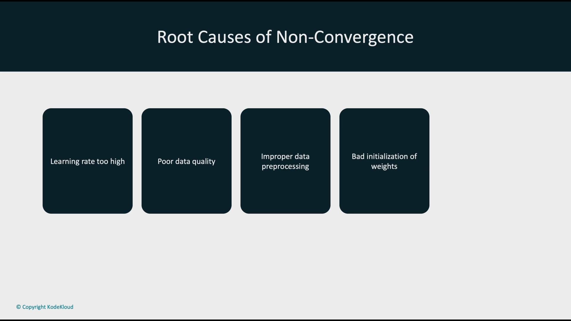
High-quality, well-preprocessed data and sensible initialization/hyperparameter choices are often the fastest way to fix convergence problems.
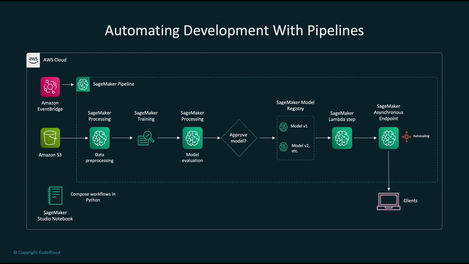
- Trigger via EventBridge schedule or when new data arrives in
Amazon S3. - SageMaker Pipelines runs a processing job to preprocess and validate data.
- A SageMaker training job trains the model using the cleaned data.
- A subsequent processing job evaluates the trained model.
- If the model meets criteria, it is approved and registered in the SageMaker Model Registry.
- An
AWS Lambdastep or a pipeline deployment step deploys the registered model to an endpoint (asynchronous or synchronous), with autoscaling for client traffic. - Clients access the deployed endpoint for inference.
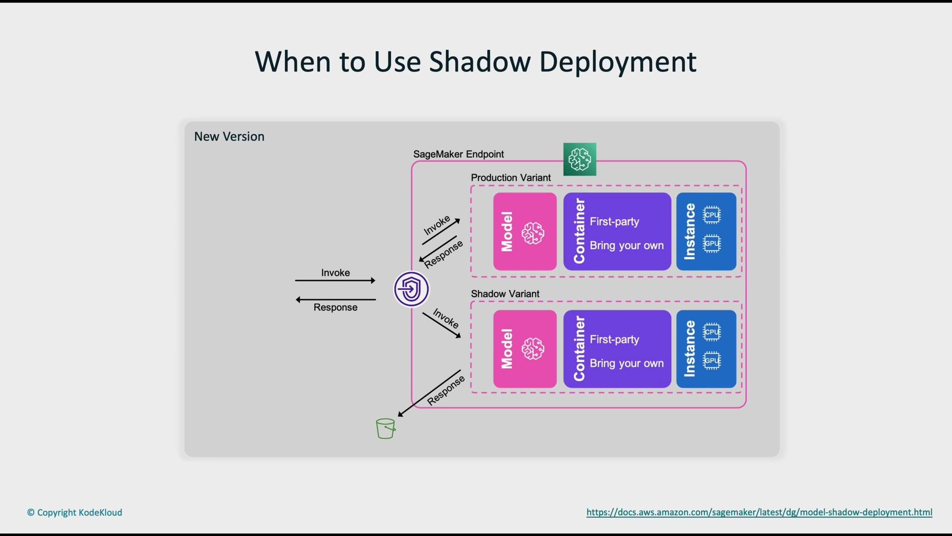
- Route user requests to the production (primary) variant as usual.
- Send a copy of each request to the shadow (candidate) variant for evaluation.
- The shadow processes requests and logs outputs for offline analysis but does not return responses to users.
- Compare shadow predictions to production behavior to detect regressions or improvements under real-world traffic patterns.
- Machine learning categories: supervised, unsupervised, and reinforcement learning.
- Good data, correct error (loss) functions, and appropriate validation are essential for effective model training and evaluation.
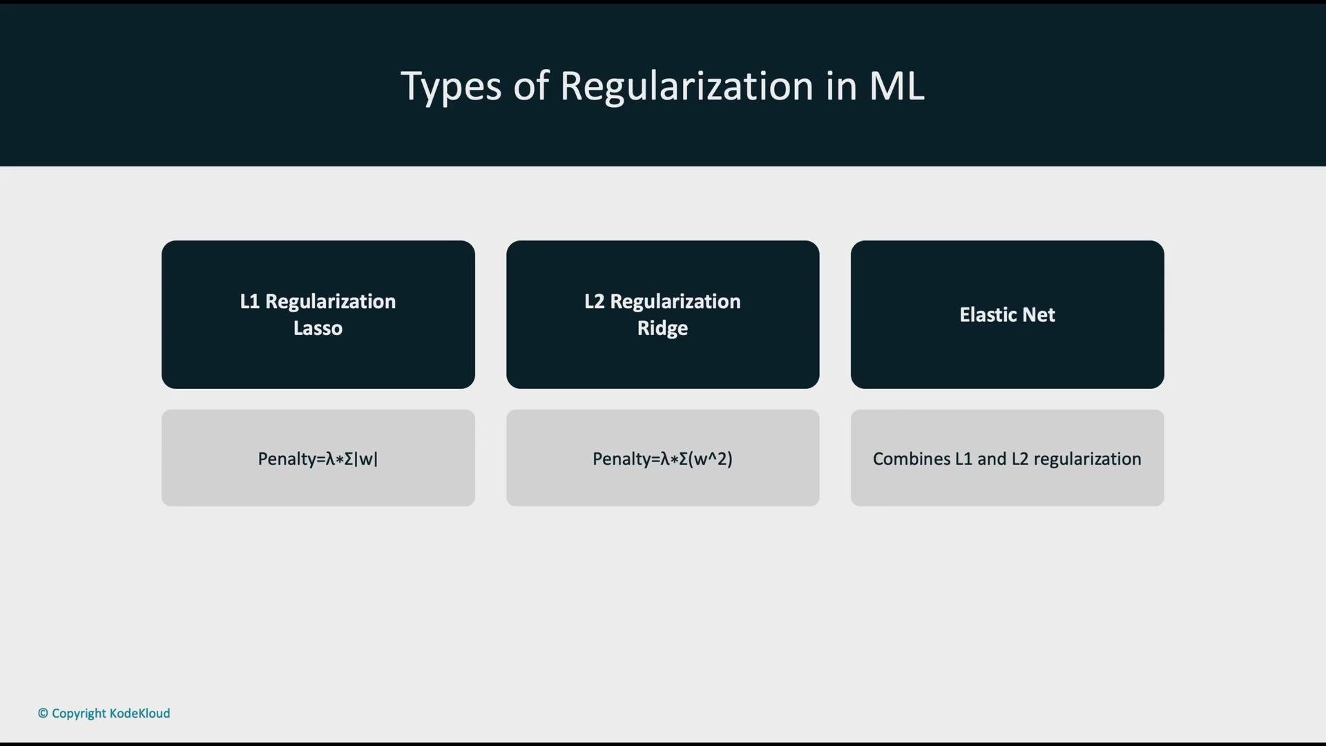
- Regularization (L1, L2, ElasticNet) helps control overfitting and shapes model sparsity and weight magnitudes.
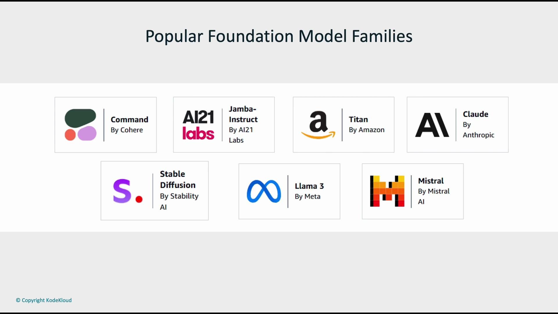
- Foundation models and pre-trained checkpoints accelerate development; fine-tuning adapts them to specific tasks.
- Address convergence issues by adjusting learning rates, improving data quality and preprocessing, using better initializations, and tuning hyperparameters.
- Production workflows include automated pipelines, model registries, safe rollout strategies (blue/green, canary, shadow), and continuous monitoring to manage drift and performance.
- Register and version models in a model registry.
- Implement approval gates (automated tests, performance thresholds).
- Use controlled rollout strategies (blue/green, canary, shadow) for safe releases.
- Monitor endpoint performance and drift; be ready to roll forward, roll back, or retrain.
- Amazon SageMaker Documentation
- Amazon S3
- AWS Lambda
- For foundational reading on model regularization and optimization: consider standard ML textbooks and the latest practitioner blogs for real-world tuning advice.