

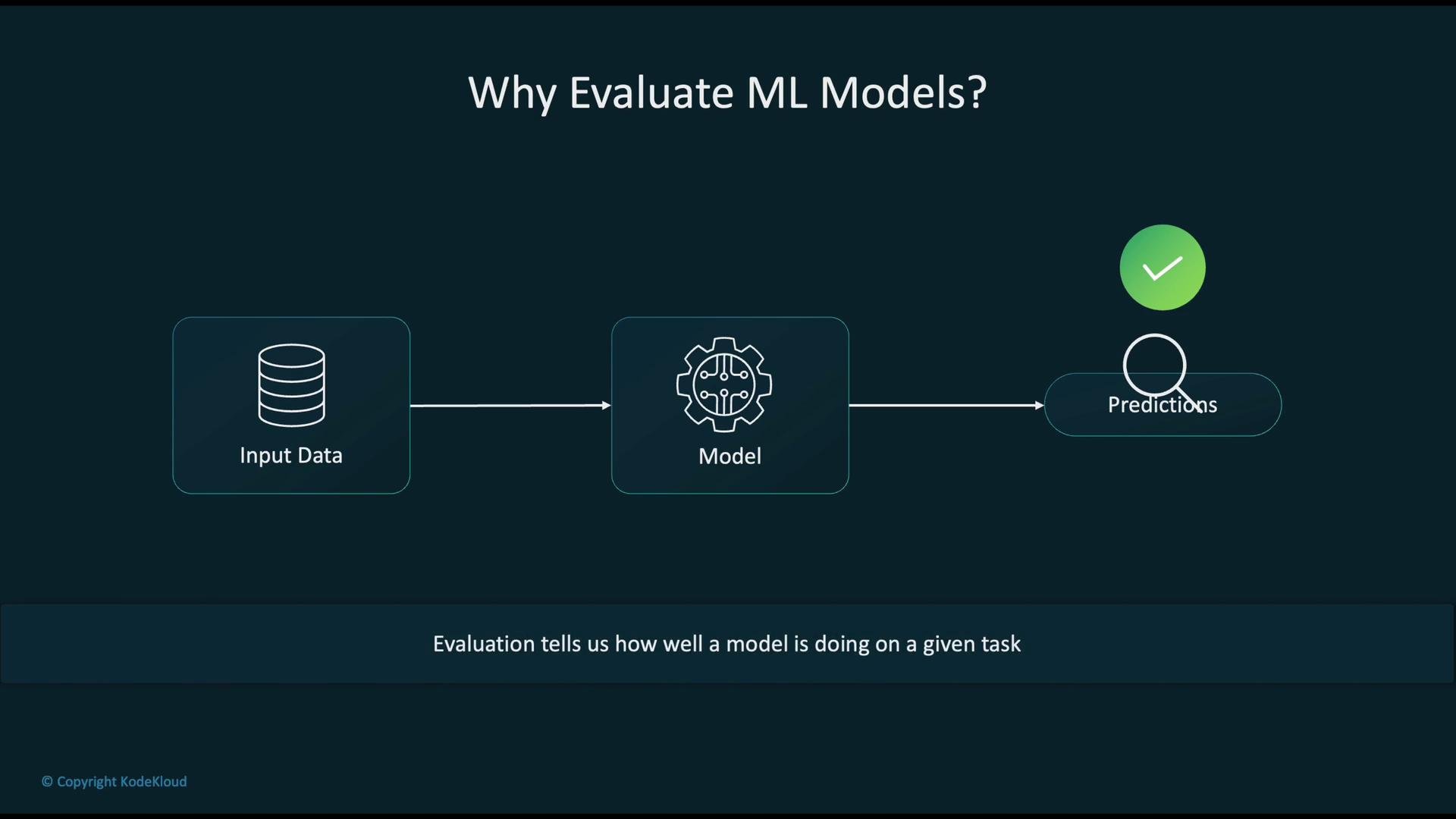
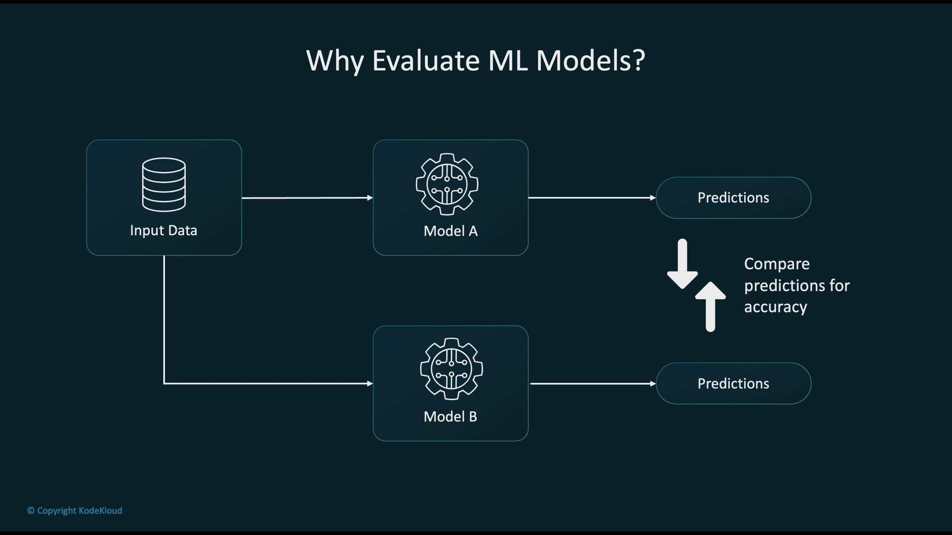
Confusion Matrix (Classification Diagnostics)
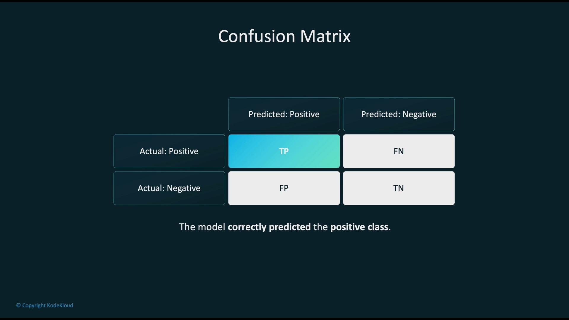
A confusion matrix decomposes binary classification outcomes into four categories:- True Positive (TP): predicted positive, actual positive
- False Negative (FN): predicted negative, actual positive
- False Positive (FP): predicted positive, actual negative
- True Negative (TN): predicted negative, actual negative
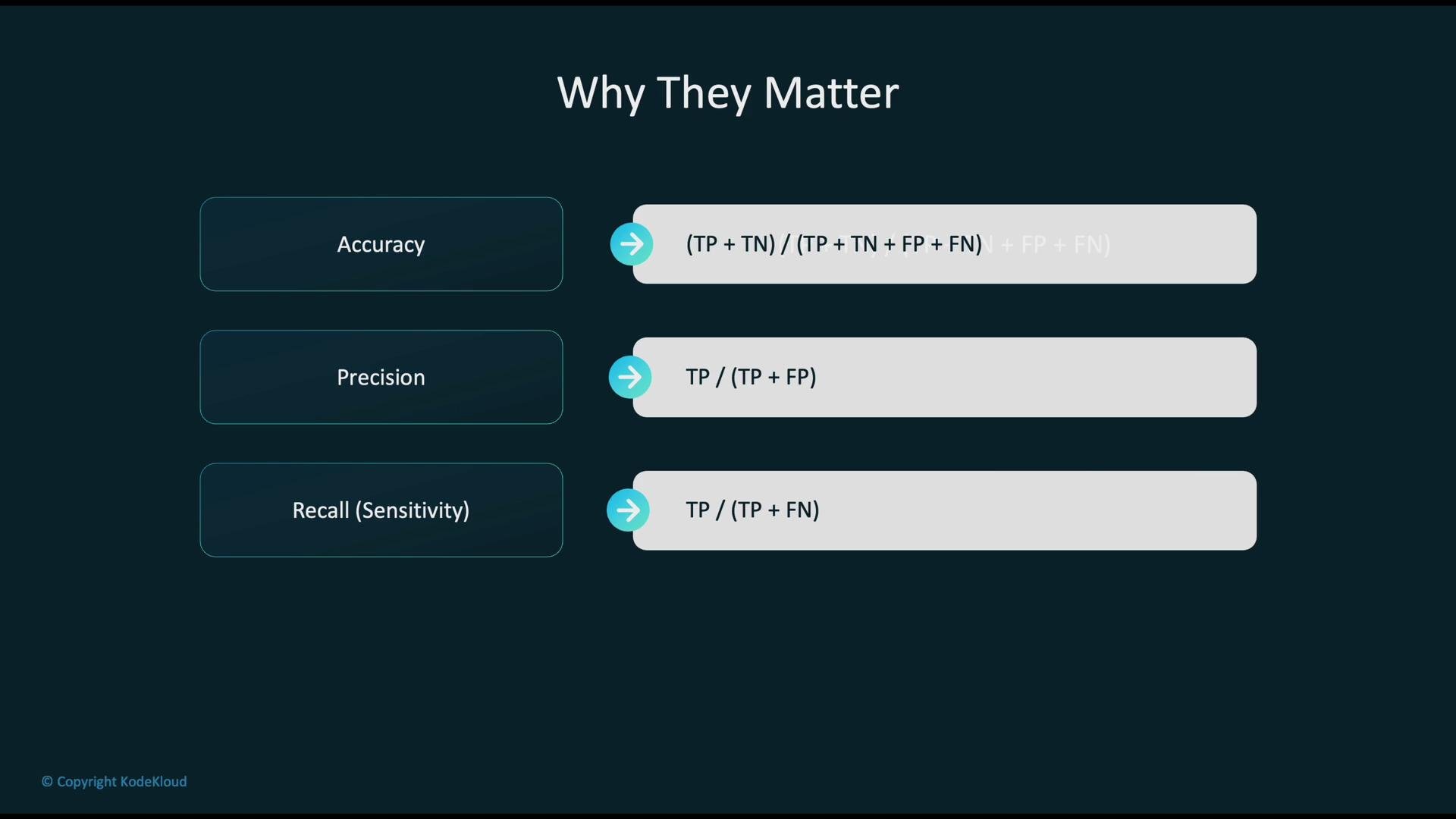
- Choose metrics that reflect business priorities: reducing false negatives vs. false positives has different operational consequences.
- For highly imbalanced datasets, avoid relying solely on accuracy.
Receiver Operating Characteristic (ROC) and AUC
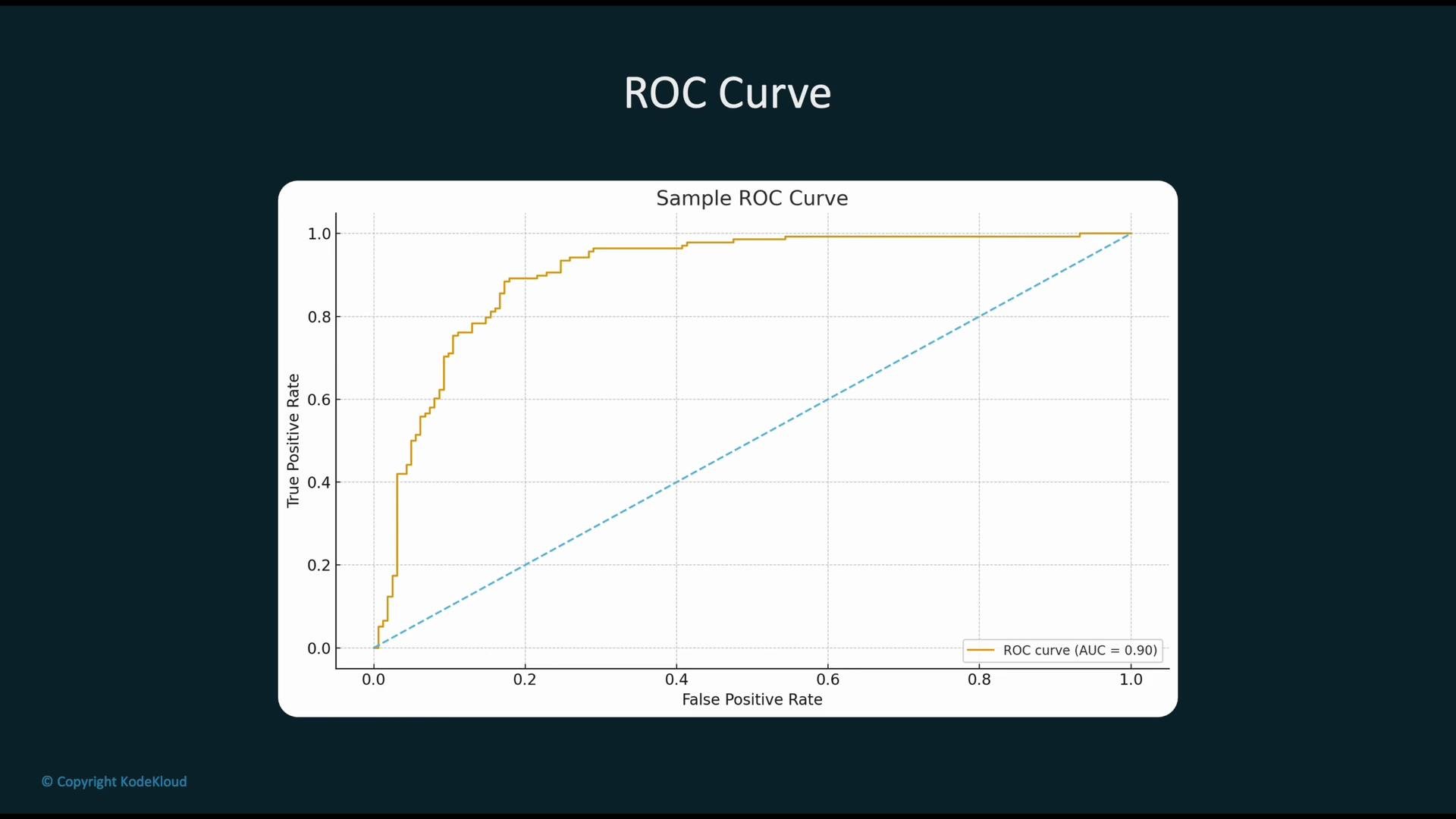
An ROC curve evaluates a classifier’s ability to separate positive and negative classes across all decision thresholds. It plots:- y-axis: True Positive Rate (TPR or Recall)
- x-axis: False Positive Rate (FPR)
Learning Curves (Bias–Variance Diagnosis)
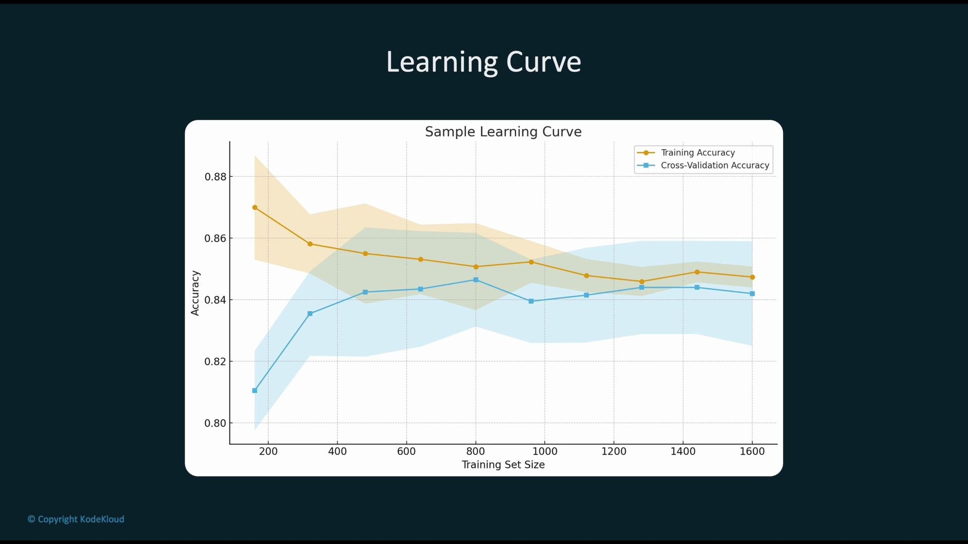
Learning curves plot model performance on training and validation (or cross-validation) sets as a function of training set size. Typical patterns:- High training score and much lower validation score => overfitting (high variance)
- Both low scores => underfitting (high bias)
- Validation score improves and plateaus as more data is added => model capacity may be adequate
Regression Metrics (Continuous Targets)
Common metrics for regression tasks include:- MAE: average absolute deviations — robust to outliers compared with MSE.
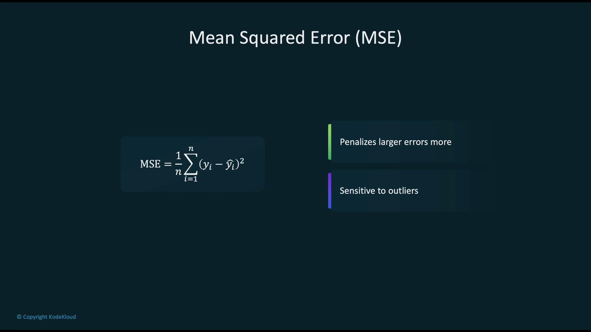
- MSE: penalizes larger errors more — useful as an optimization objective.
- RMSE: same units as the target — easier to interpret.
- R^2: fraction of variance explained; values near 1 are good, 0 indicates performance equivalent to predicting the mean, and negative values indicate worse than the mean predictor.
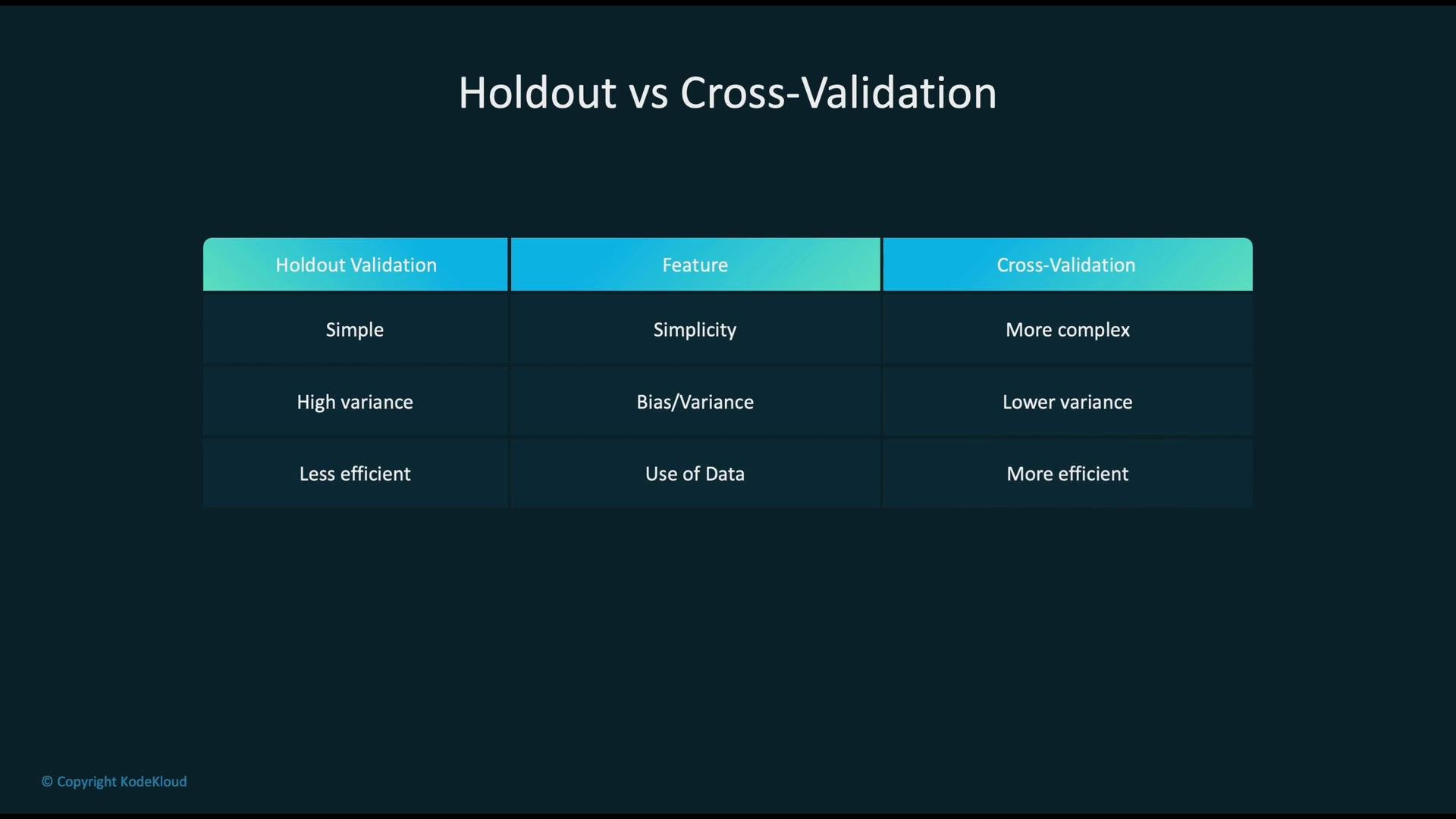
Validation Strategies (Holdout vs. Cross-Validation)
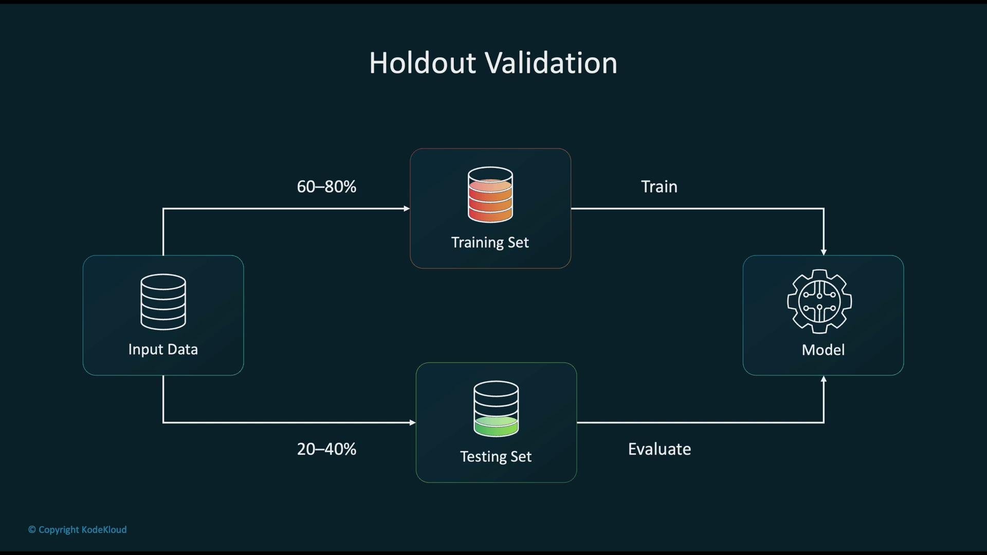
Holdout Validation:- Split the dataset into distinct subsets:
- Training set: ~60–80% — used to train the model.
- Test set: ~20–40% — used to evaluate final performance.
- Optional validation set: held out from the training split for hyperparameter tuning.
- Pros: simple and fast; works well on large datasets.
- Cons: higher variance in estimates if dataset is small.
- Split data into
kfolds (commonlyk = 5ork = 10). - For each fold: train on
k-1folds and validate on the remaining fold. - Average metrics across folds for a more robust estimate.
- Reduces evaluation variance and is especially valuable with limited data.
- Holdout: large datasets, need quick iteration.
- Cross-validation: limited data or when you need stable, lower-variance estimates.
Practical Tooling and Monitoring (AWS)
AWS offers services to help evaluate, monitor, and detect issues in models:- Amazon CloudWatch: capture logs, metrics, and alerts for training jobs and deployed endpoints.
- Amazon SageMaker Clarify: bias detection, feature importance, and dataset imbalance reporting.
- Amazon SageMaker Training Metrics: record accuracy, loss, and custom metrics during training.
Choose evaluation metrics and validation strategies that match your business goals and the risks of each type of error. For imbalanced problems, prefer precision/recall or AUC-PR and consider cross-validation to get stable estimates.
- Scikit-learn: Model evaluation — https://scikit-learn.org/stable/modules/model_evaluation.html
- ROC curve and AUC — https://en.wikipedia.org/wiki/Receiver_operating_characteristic
- Amazon SageMaker Clarify — https://docs.aws.amazon.com/sagemaker/latest/dg/clarify.html
- Amazon CloudWatch — https://aws.amazon.com/cloudwatch/