Model Size Reduction Techniques

Modern large language models (LLMs) can exceed one trillion parameters and often need dozens to hundreds of GPUs to run efficiently. Many target platforms—phones, IoT devices, drones, and wearables—have limited memory, compute power, and energy. This article explains why model size reduction matters, the most common techniques for compressing models, and how to select and validate methods that fit your deployment constraints.

The image lists scenarios that need size reduction, including phones, IoT devices, drones, and wearables, with a focus on limited memory.

Why model size reduction matters

Reduced memory footprint: Fit models on-device or into smaller cloud instances.
Faster inference: Lower compute cost and reduced latency for real-time applications.
Lower infrastructure cost: Smaller models reduce CPU/GPU time and energy consumption.
Offline usage: Enable functionality without persistent network connectivity.
Easier distribution and updates: Smaller artifacts are faster to transfer and deploy.

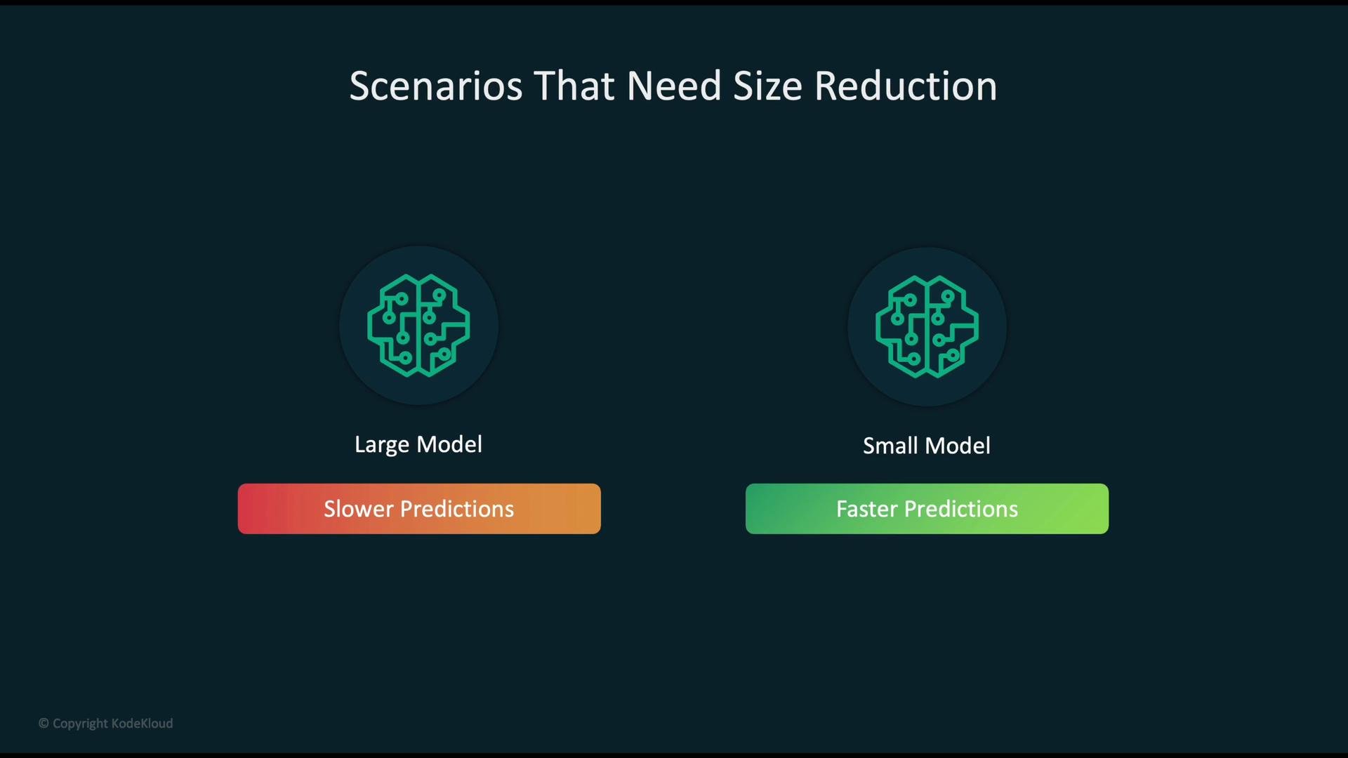
Because large models require more computation, they often produce slower predictions. Latency is critical for many real-time applications—on-device AR, robotics, and mobile assistants—so compressing and optimizing models is essential.

The image illustrates a comparison between large and small models, highlighting that large models have slower predictions while small models have faster predictions.

Common deployment motivations

Deploy to edge and mobile devices
Improve inference throughput and latency
Reduce cloud infrastructure cost
Support offline/low-bandwidth scenarios
Accelerate fine-tuning and iterative development

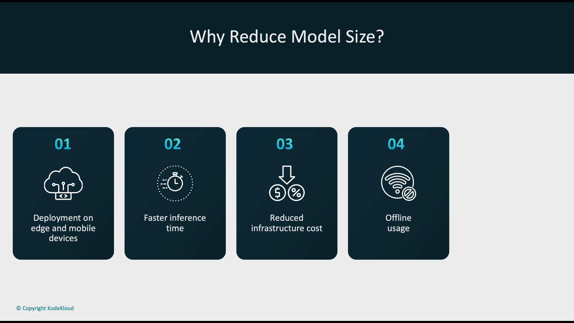
The image presents four reasons for reducing model size: deployment on edge and mobile devices, faster inference time, reduced infrastructure cost, and offline usage.

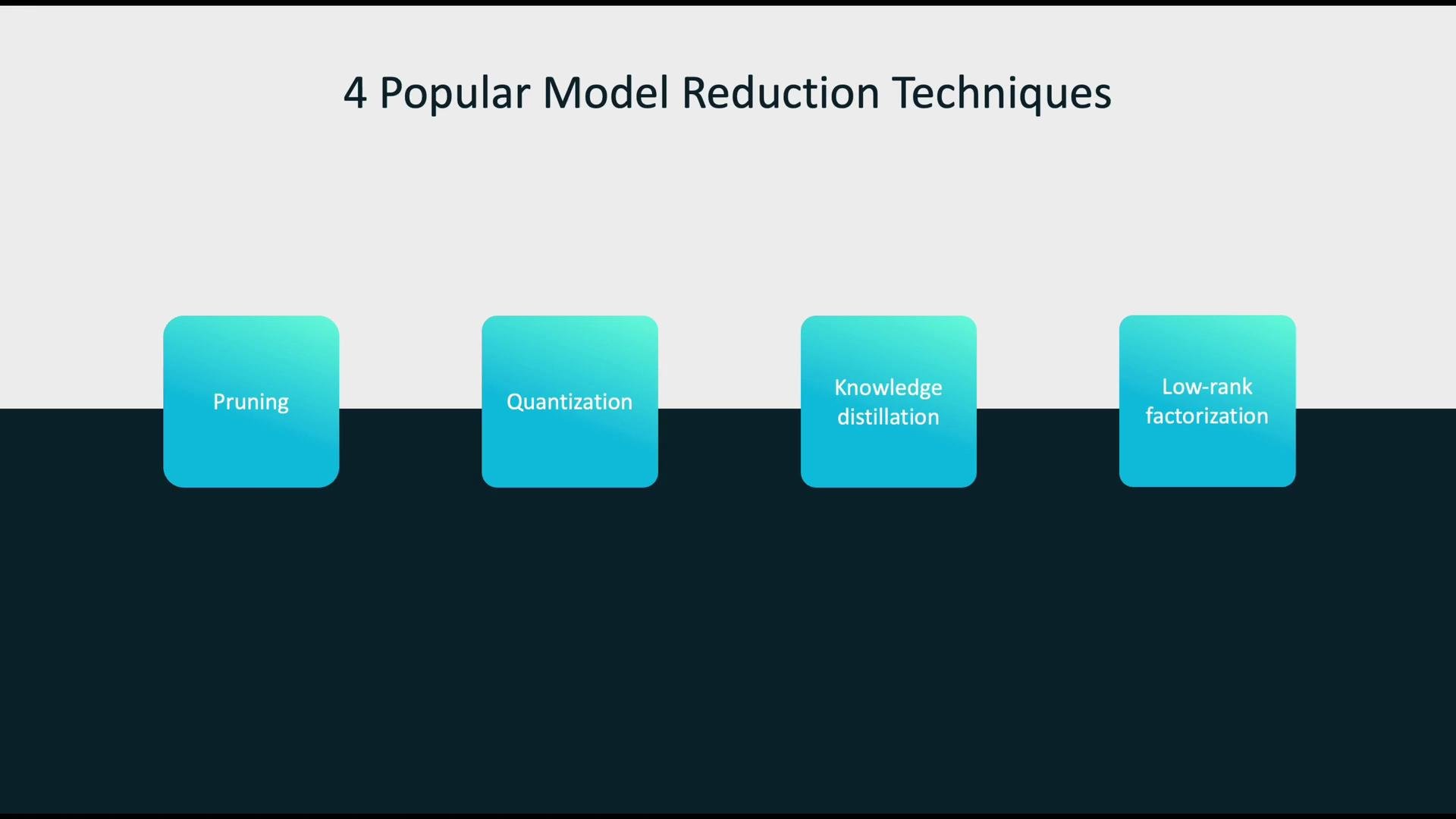
Overview of popular model-reduction techniques

Pruning
Quantization
Knowledge distillation
Low-rank factorization

The image lists four popular model reduction techniques: pruning, quantization, knowledge distillation, and low-rank factorization.

Pruning Pruning removes redundant or low-importance weights, neurons, or filters from a network to reduce parameter count and computation. Typical pruning strategies include:

Magnitude pruning: drop small-magnitude weights.
Structured pruning: remove entire neurons, channels, or filters for hardware-friendly sparsity.
Iterative pruning and retraining: prune gradually and fine-tune to recover accuracy.

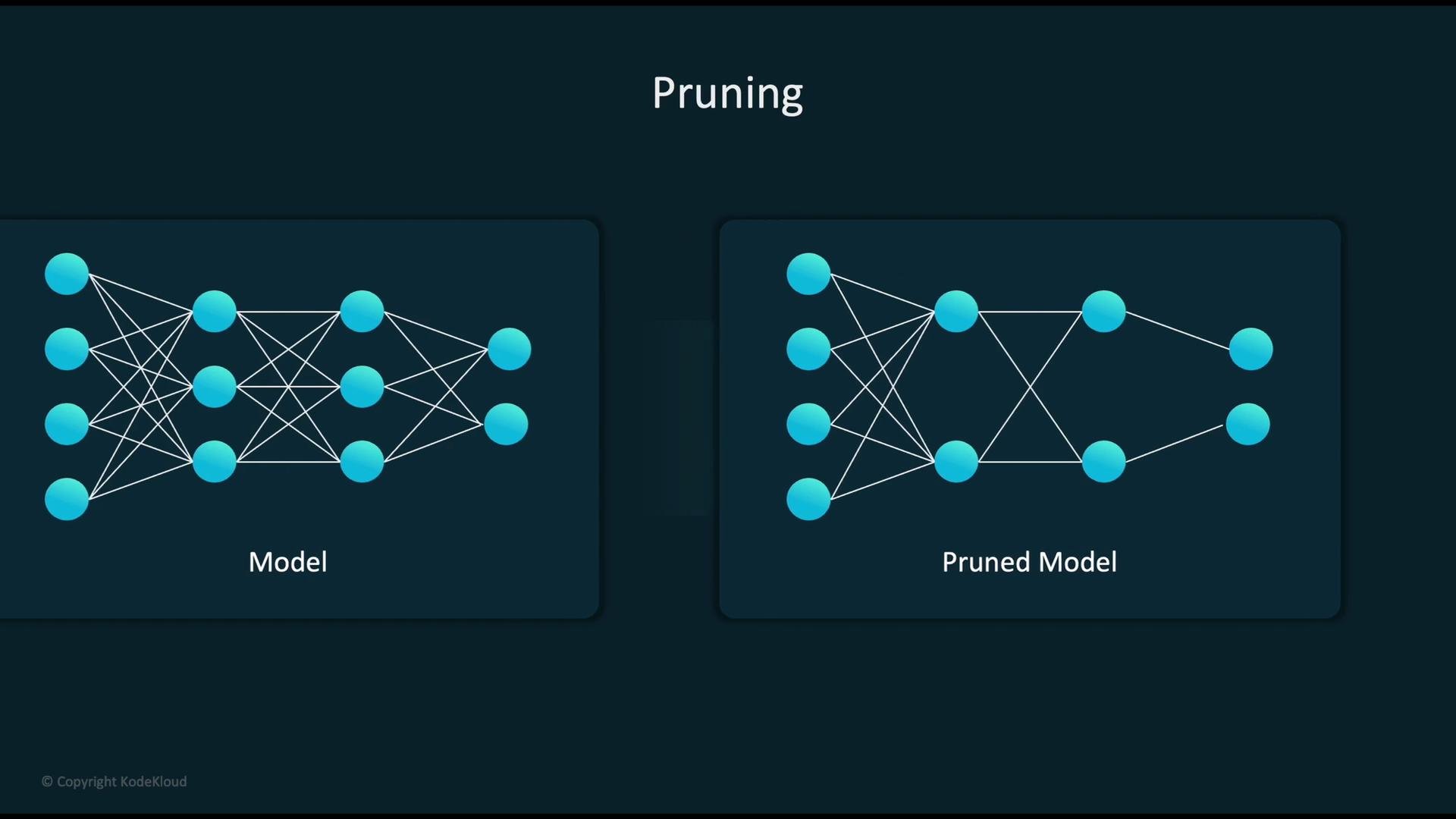
Pruning usually reduces both storage and runtime cost, but it commonly requires a fine-tuning step to regain performance.

The image shows a comparison between a neural network model and its pruned version, illustrating how pruning reduces the number of connections and nodes.

Quantization Quantization reduces numerical precision of model weights and/or activations, shrinking model size and often speeding up inference on CPUs, some GPUs, and accelerators. Common quantization options:

FP16 (half precision): often minimal accuracy loss, widely used on GPUs.
INT8 (8-bit integer): much smaller footprint and faster CPU inference; often needs calibration or quantization-aware training.
Dynamic (post-training) quantization: convert weights on the fly with no calibration data.
Static (calibrated) quantization: uses calibration dataset to determine ranges.
Quantization-aware training (QAT): simulates quantization during training to preserve accuracy.

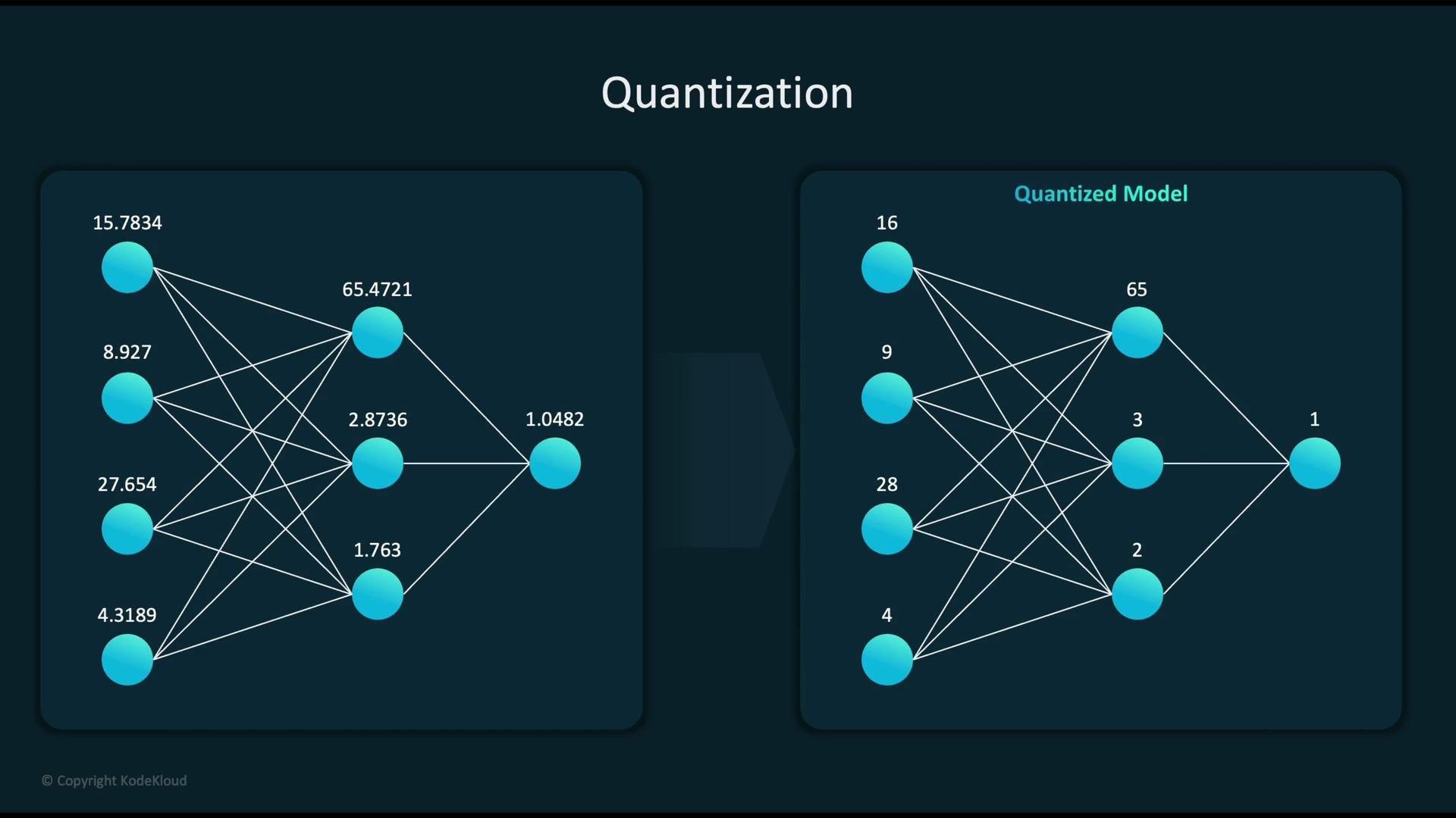
Always evaluate post-quantization accuracy and latency on the target hardware.

The image illustrates the concept of quantization in neural networks, showing a comparison between a regular model and a quantized model with simplified numerical values.

Knowledge distillation Knowledge distillation transfers behavior from a large (teacher) model to a smaller (student) model. Instead of training the student purely on hard labels, the student learns to match the teacher’s soft output distributions—this can encode richer information about class similarities and calibration. Key points:

Can produce compact models that retain much of the teacher’s capability.
Often combines distillation loss with label loss.
Commonly used for both classification and generative tasks.
Requires additional training of the student model.

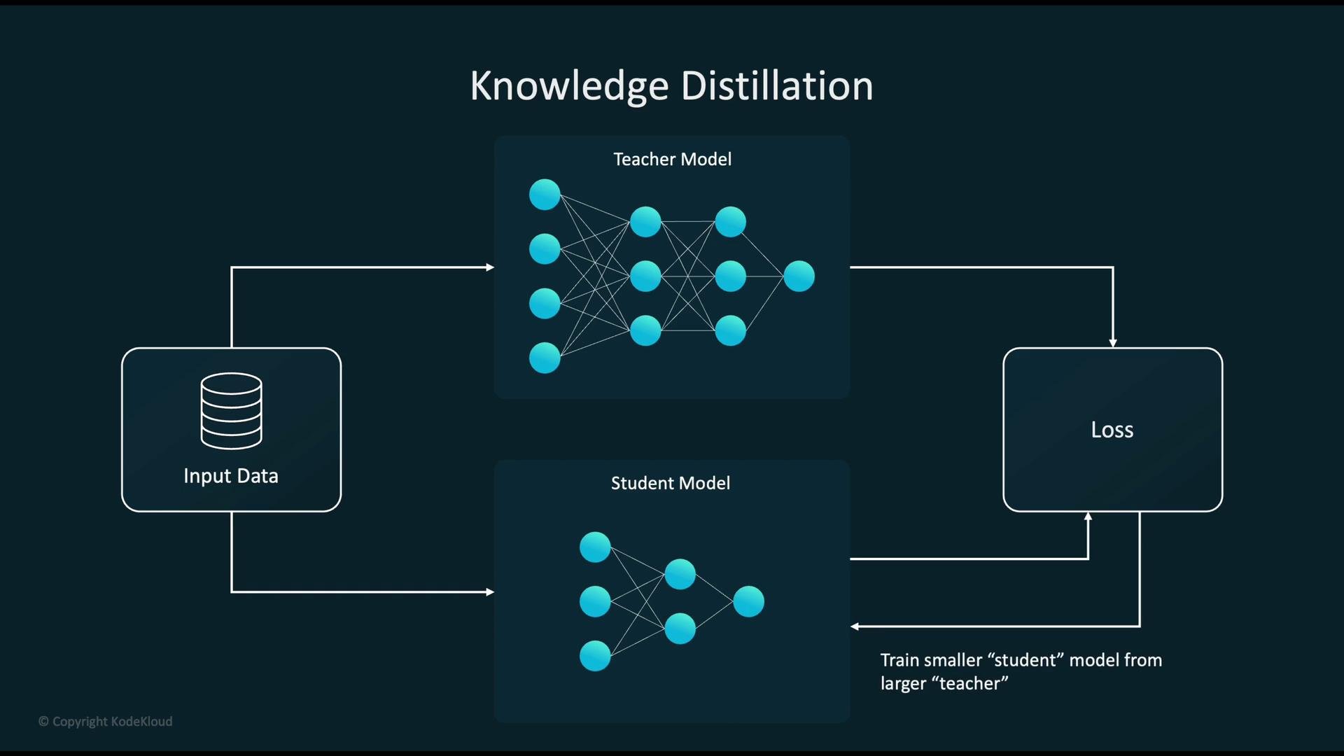
The image illustrates a knowledge distillation process, showing input data being fed into a teacher model and a smaller student model with a loss function to optimize the training.

Low-rank factorization Low-rank factorization approximates large weight matrices as products of smaller matrices to reduce both storage and multiply-add cost. For a matrix A (m × n), approximate: A ≈ U (m × k) × V (k × n) with k < min(m, n). Choosing k trades off accuracy vs. parameter count. A common approach to compute a low-rank approximation is truncated singular value decomposition (SVD). Example using NumPy:

import numpy as np

# Example matrix A (3x3)
A = np.array([
    [1.0, 4.0, 7.0],
    [1.0, 5.0, 8.0],
    [1.0, 6.0, 10.5]
])

# Compute full SVD
U_full, S_full, Vt_full = np.linalg.svd(A, full_matrices=False)

# Choose rank k = 2 for approximation
k = 2
U_k = U_full[:, :k]
S_k = np.diag(S_full[:k])
Vt_k = Vt_full[:k, :]

# Reconstruct rank-k approximation
A_k = U_k @ S_k @ Vt_k

print("Original A:\n", A)
print("\nRank-{} approximation A_k:\n".format(k), A_k)

The truncated singular values indicate component importance; small singular values can often be discarded with limited downstream impact. Recap: technique trade-offs

Technique	What it reduces	Pros	Cons / Considerations
Pruning	Parameters & compute	Can give large size reductions; structured variants are hardware-friendly	Often requires iterative retraining and careful sparsity patterns
Quantization	Precision & storage	Major size and latency wins on supported hardware	Possible accuracy loss; needs calibration or QAT
Distillation	Model capacity	Produces small, high-quality student models	Requires additional training and dataset passes
Low-rank factorization	Matrix size & computation	Reduces FLOPs for dense layers; mathematically principled	Rank selection affects accuracy; not always best for attention layers

Choosing the right combination depends on model architecture, deployment hardware, and acceptable accuracy trade-offs. In practice, teams combine techniques—e.g., distill a student model, then quantize it and apply light pruning.

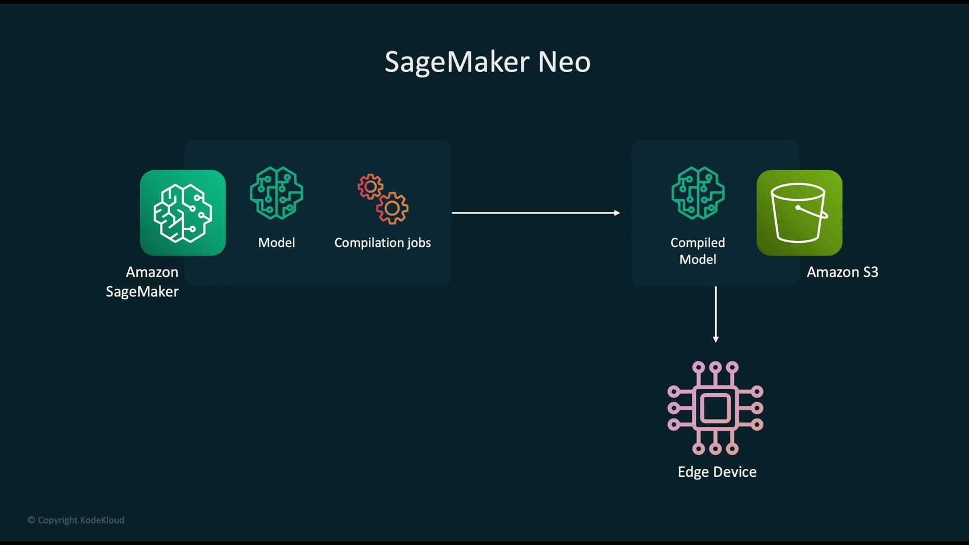
The image illustrates the workflow of Amazon SageMaker Neo, showing the process from creating a model with Amazon SageMaker, through compilation jobs, to deploying a compiled model to Amazon S3 and an edge device.

SageMaker Neo (concept) A trained model from Amazon SageMaker can be sent to a compilation job where SageMaker Neo produces a hardware-optimized compiled model. The optimized artifact can be stored in Amazon S3 and deployed to edge devices or specific environments. This workflow enables the same model logic to run faster with lower latency on target hardware without manual low-level optimizations.

SageMaker Neo docs: https://docs.aws.amazon.com/sagemaker/latest/dg/sagemaker-neo.html
Amazon SageMaker: https://aws.amazon.com/sagemaker/
Amazon S3: https://aws.amazon.com/s3/

Best practices

Understand trade-offs — measure compression impact on accuracy, latency, and memory. Prioritize metrics that matter for your product (e.g., 95th percentile latency vs. mean latency).
Match technique to hardware — structured pruning and INT8 quantization are often better supported on edge CPU/GPU/ISP stacks.
Iterate and tune — sweep pruning rates, quantization schemes, distillation temperatures, and rank k values to find the best balance.
Profile on target device — benchmarks on simulators or desktops can differ from real hardware due to memory hierarchy and instruction set differences.
Regularize during training — weight decay, dropout, and early stopping improve robustness to compression.
Combine methods carefully — distill first, then quantize and prune lightly; verify end-to-end accuracy and latency.

When evaluating compressed models, always benchmark real-world inference latency and accuracy on the target device. Simulator or desktop measurements can differ from on-device behavior.

Beware: aggressive compression (very low rank, extreme pruning, or INT8 quantization without calibration) can cause unacceptable accuracy degradation. Validate thoroughly and keep rollback plans for production deployments.

Links and references

Watch Video

Ensemble Learning Methods

Demo Model Version Management with SageMaker Model Registry

Prerequisites

Data Preparation for Machine Learning (ML)

ML Model Development

Deployment and Orchestration of ML Workflows

ML Solution Monitoring, Maintenance, and Security

Bringing it all together

Model Size Reduction Techniques

Watch Video