

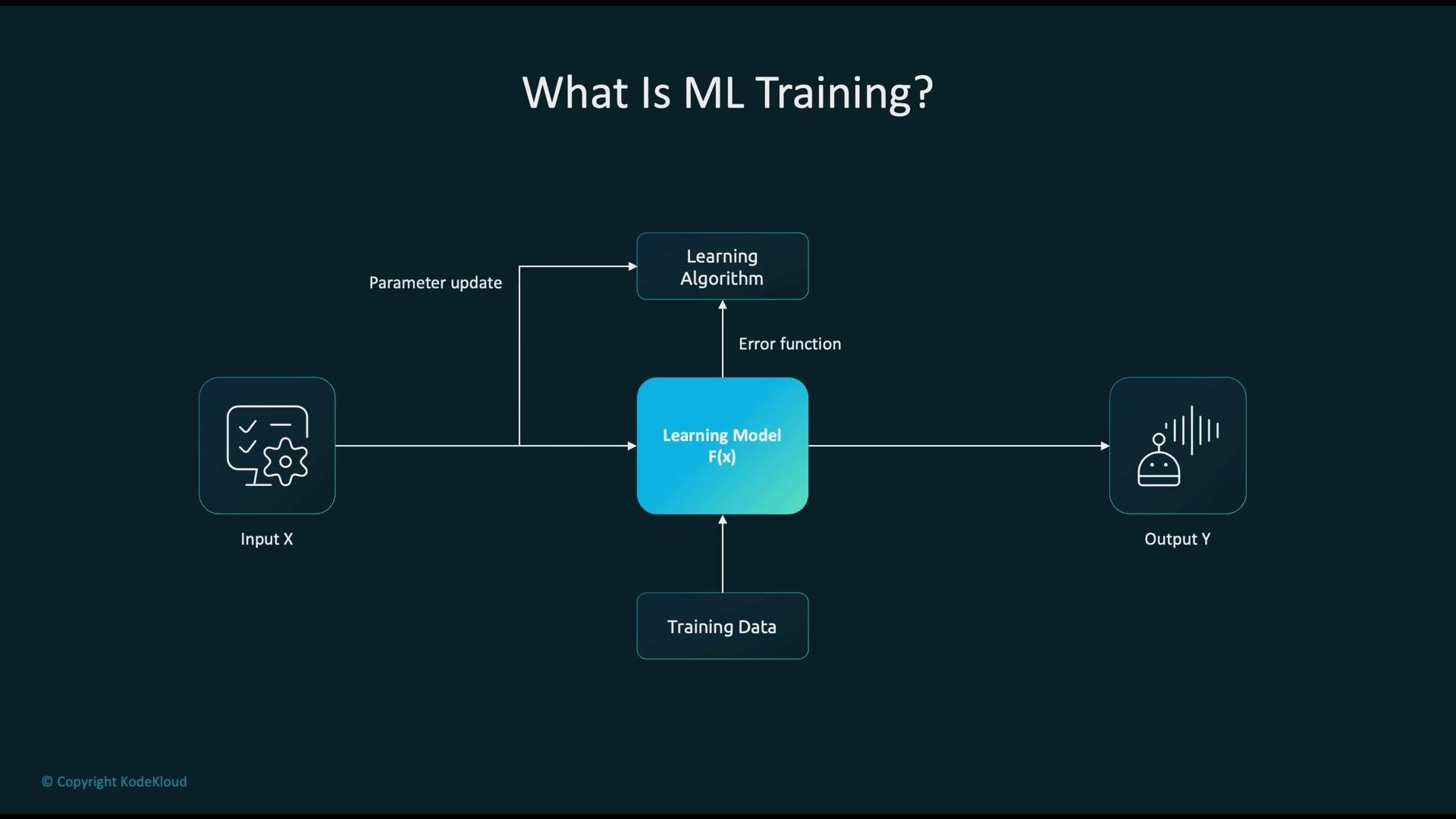
x (a feature or data point) through a function f(x) to produce a prediction y_hat that approximates the true label y. Training adjusts model parameters so predictions align with real outcomes.
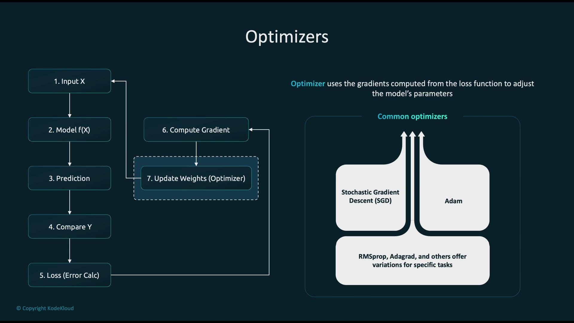
Key components of a training loop include labeled training data, a learning algorithm to adjust parameters, a loss function to quantify error, and an optimizer to update parameters using gradients computed from the loss.
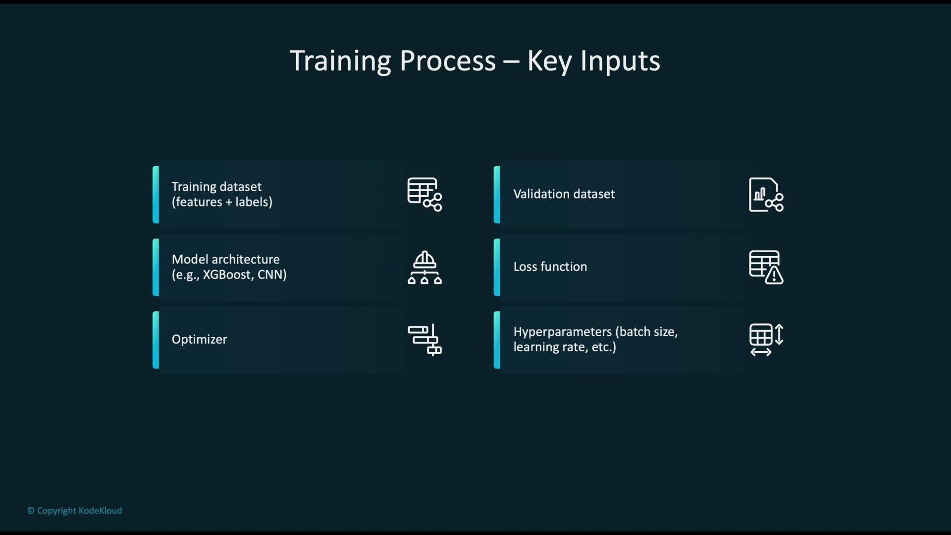
- A training dataset (features + labels).
- A validation dataset (and ideally a separate test dataset) for evaluation.
- A chosen model architecture (e.g., XGBoost, CNN).
- A loss function that quantifies prediction error.
- An optimizer to update model parameters.
- Hyperparameters such as learning rate, batch size, and number of epochs.
Data splitting and validation
To evaluate generalization, datasets are typically partitioned into training and validation/test sets. A common heuristic is to allocate roughly 80% of data to training and 20% to validation/testing; however, the exact split depends on dataset size and domain constraints. Cross-validation is another common strategy to make efficient use of limited data.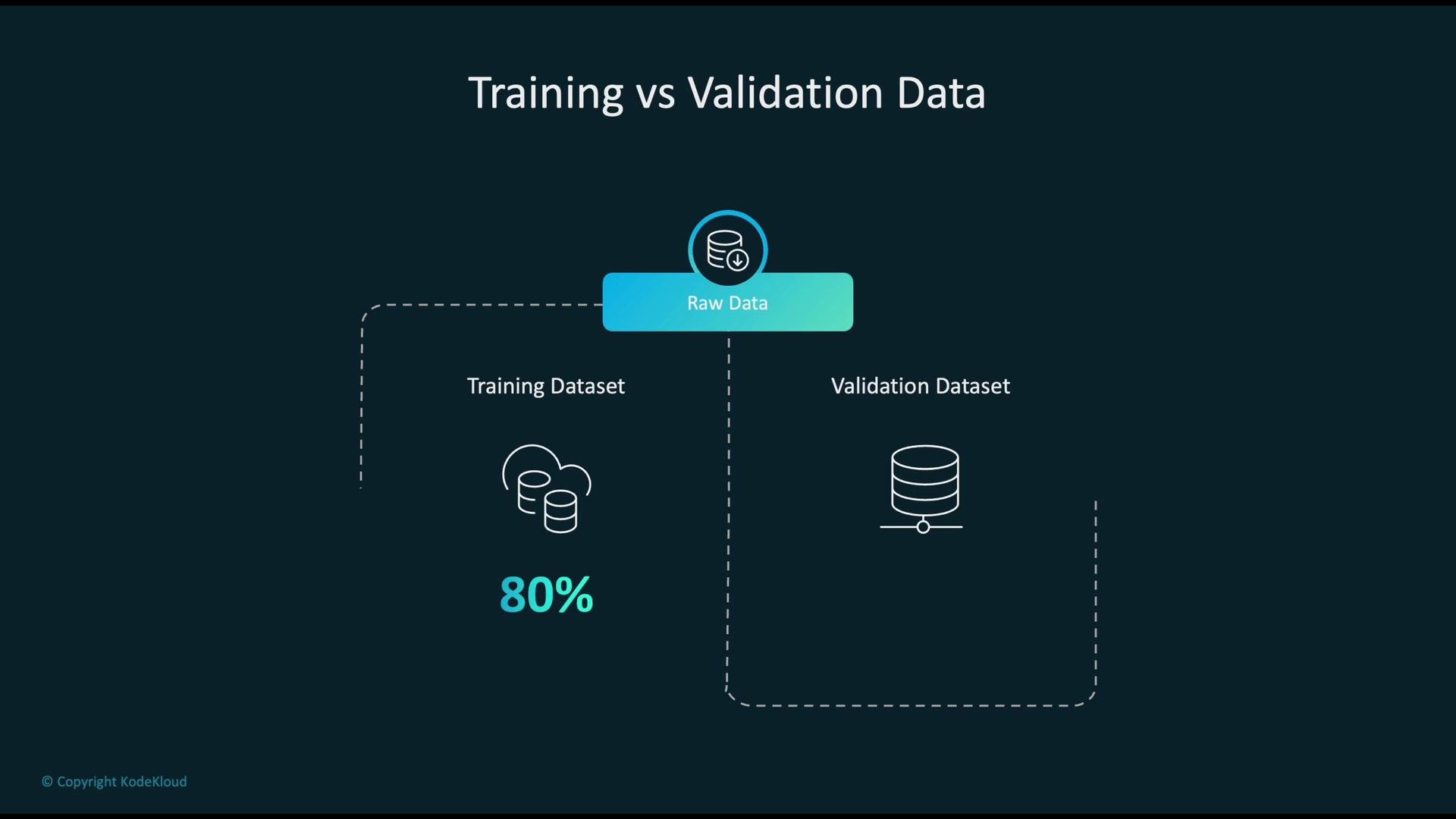
Training loop: forward and backward passes
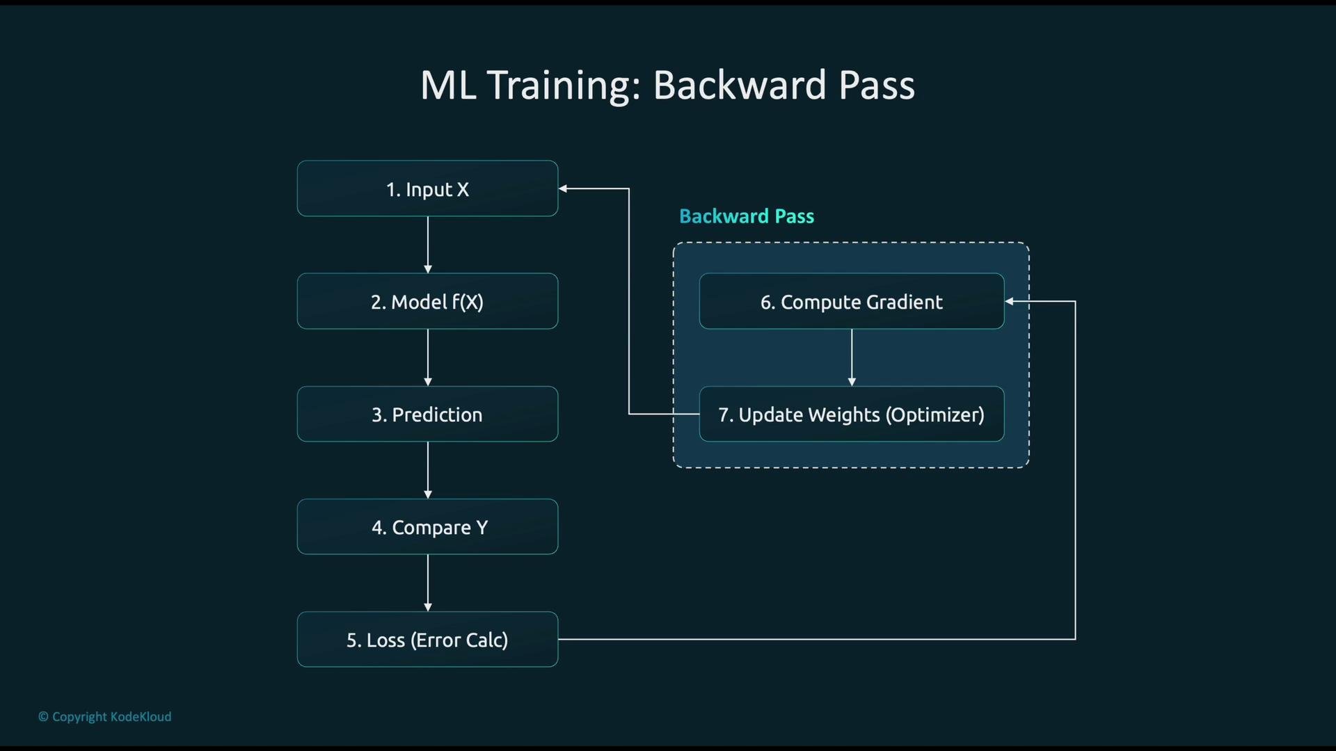
A typical training iteration performs the following steps:- Input
X— the features or data points. - Forward pass through the model
f(x)to produce predictionsy_hat. - Compare predictions with true labels
y. - Compute the loss using a chosen loss function.
- Compute gradients of the loss with respect to model parameters (backpropagation).
- Optimizer updates parameters using the gradients.
- Repeat across batches and epochs until convergence or stopping criteria are met.
Loss functions — measuring prediction error
Loss functions quantify how far predictions are from true values and guide parameter updates. Choose a loss that matches your task (regression vs classification) and the sensitivity you want to outliers. Common regression losses:- Absolute Error for a single data point:
|y_hat - y| - Mean Absolute Error (MAE) for
npoints:
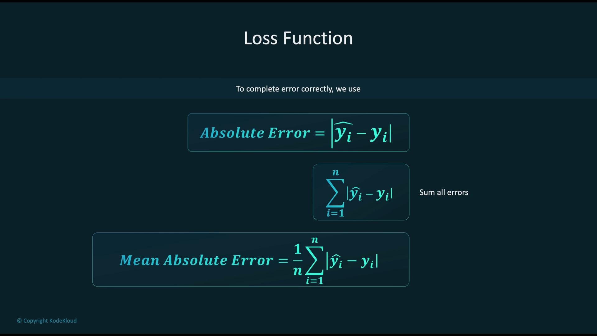
- Mean Squared Error (MSE):
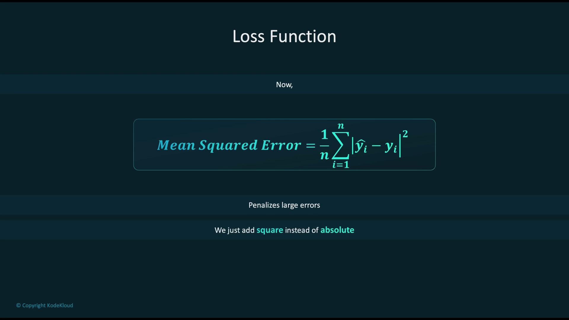
- Binary Cross-Entropy (log loss) for binary classification: penalizes confident but incorrect probability estimates.
- Categorical Cross-Entropy (paired with softmax) for multi-class classification: generalizes binary cross-entropy to multiple classes.
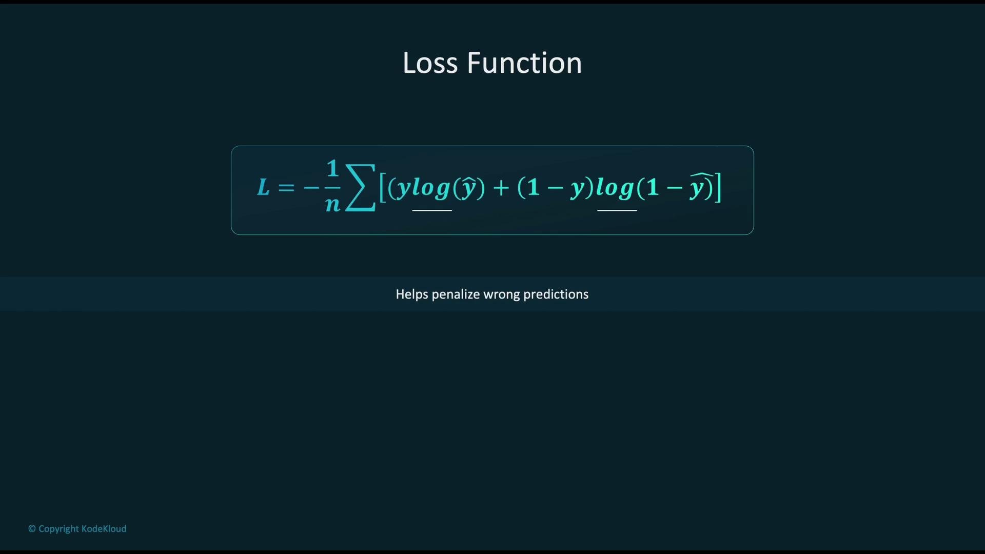
Choose the loss function that matches your task (regression vs classification) and the scale/sensitivity you want for errors (e.g.,
MAE vs MSE). Consider robustness to outliers and the effect on gradient magnitudes when selecting a loss.Optimizers — updating parameters
Optimizers use gradients from the loss to update model parameters and reduce error over training. Selection of an optimizer and its hyperparameters (e.g., learning rate) can greatly affect convergence speed and final performance. Common optimizers:- Stochastic Gradient Descent (SGD): simple, updates parameters using estimated gradients (often per batch); can be noisy but may generalize well.
- Momentum-based methods: accelerate convergence by accumulating past gradients (e.g., SGD with momentum).
- Adam: combines momentum and per-parameter adaptive learning rates for faster, often robust convergence.
- Adagrad, RMSprop: adaptive learning-rate methods suitable for sparse or non-stationary problems.
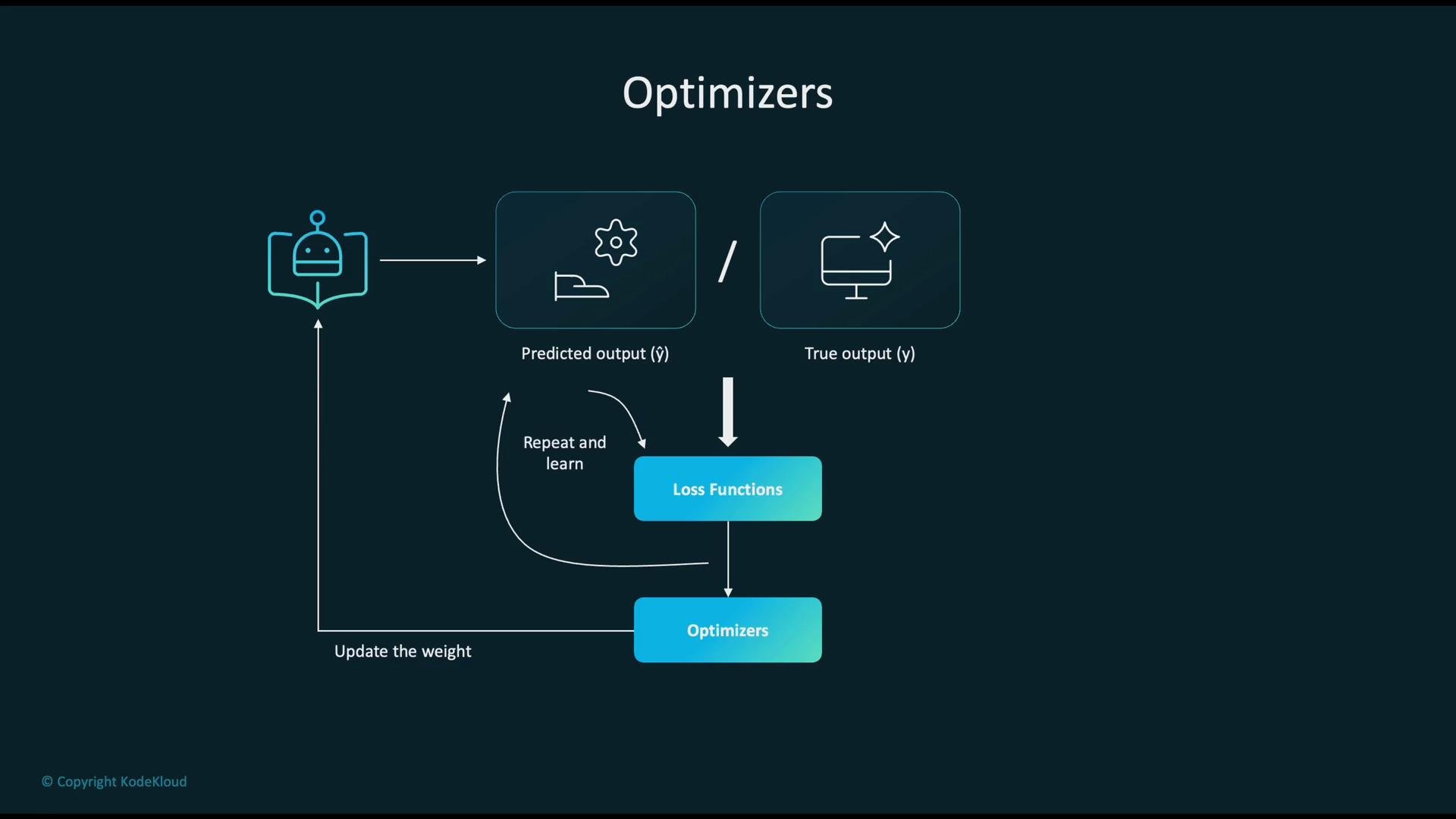
Gradient descent variants
Gradient descent is the foundation of most optimizers. Variants:- Batch Gradient Descent: compute gradients over the whole dataset (stable but slow for large datasets).
- Stochastic Gradient Descent (SGD): update using one sample at a time (fast but noisy).
- Mini-batch Gradient Descent: compute gradients on small batches — most commonly used in practice.
\theta_t are parameters at step t, \eta is the learning rate, and \nabla_{\theta} L is the gradient of the loss with respect to parameters.
Common training terms
- Epoch: one complete pass through the entire training dataset.
- Batch: a subset of the dataset processed together in one forward/backward pass.
- Iteration: one parameter update (i.e., processing one batch). Iterations per epoch =
dataset_size / batch_size.
Don’t confuse iterations and epochs: an iteration performs one parameter update on a batch, while an epoch processes the entire dataset once (many iterations per epoch).
- Kubernetes Basics (useful for deploying models)
- TensorFlow Guide
- PyTorch Documentation
- Scikit-learn User Guide