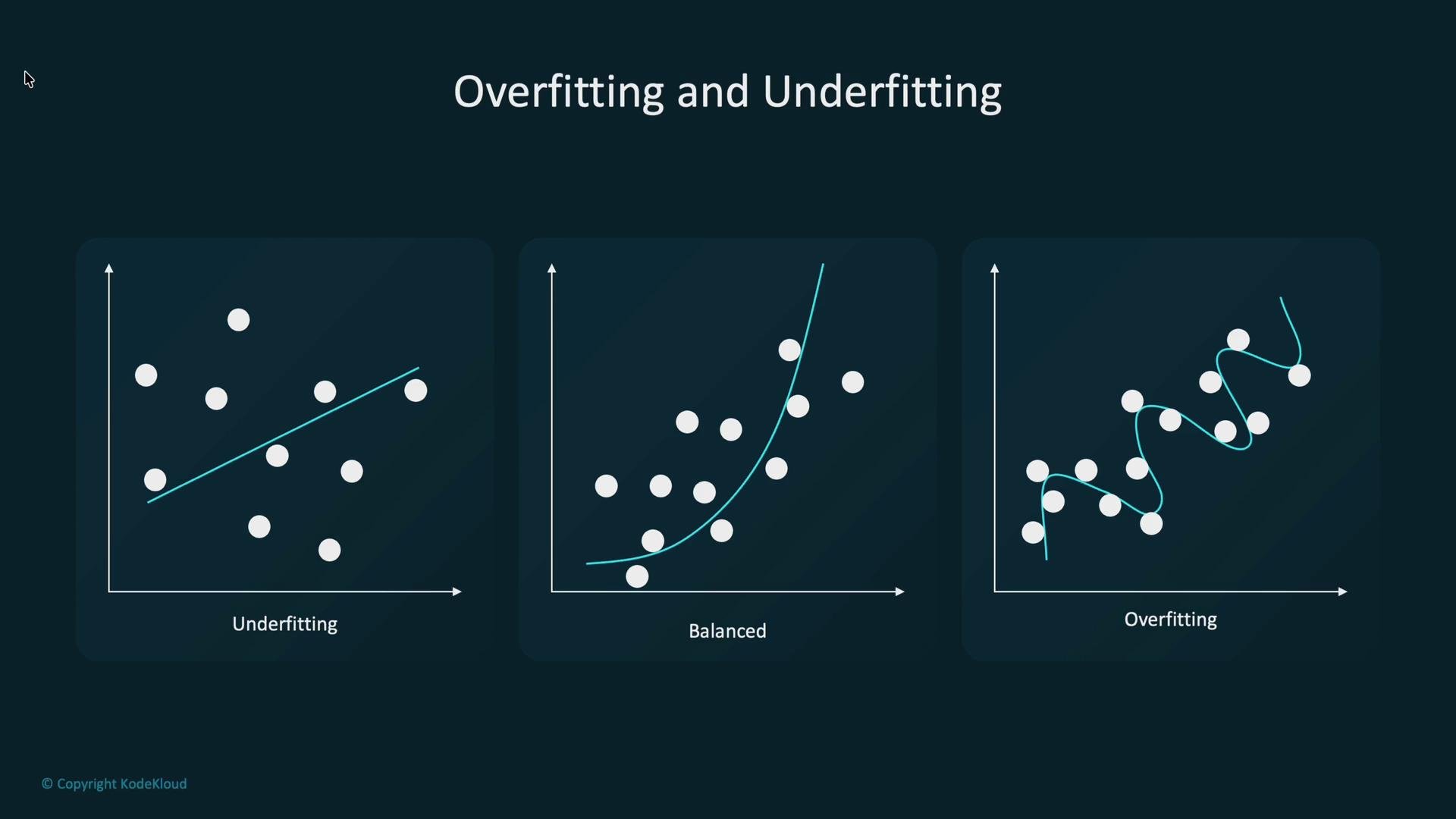
Underfitting happens when a model is too simple to capture the underlying patterns in the data, producing poor performance on both training and test sets. Overfitting occurs when a model learns the training data — including noise and outliers — so well that it fails to generalize to unseen data. The goal of regularization is to find a balanced model that generalizes well: not too simple (underfitting) and not overly complex (overfitting).
The image illustrates three graphs showing examples of underfitting, balanced fitting, and overfitting in data modeling. Each graph depicts a different type of line fitting a set of white data points.
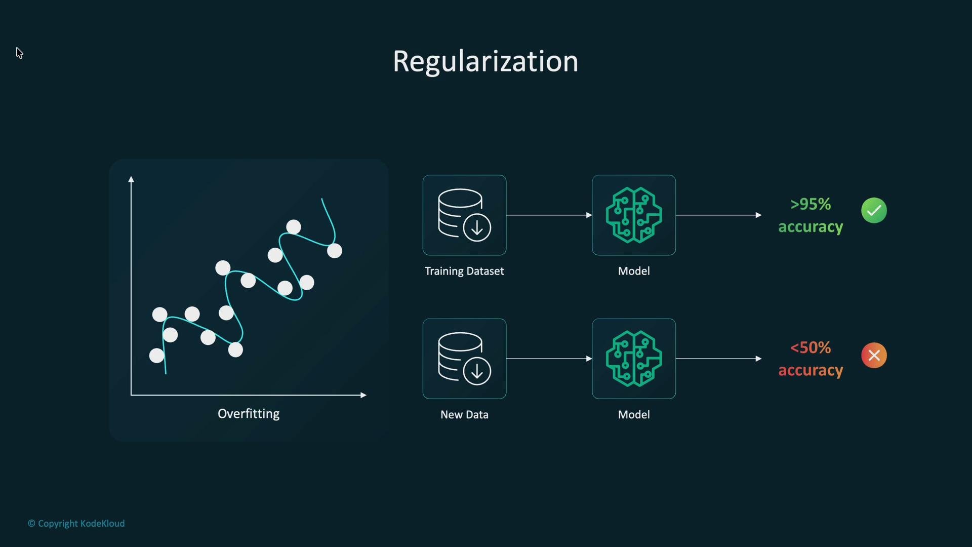
Regularization is a group of techniques that discourage overly complex models by adding a complexity penalty to the loss function. This penalty nudges model parameters toward smaller values or sparsity, improving generalization on unseen data.
The image illustrates the concept of regularization in machine learning, showing a model that overfits on a training dataset leading to high in-sample accuracy but low accuracy on new data, suggesting poor generalization.
How regularization modifies the loss function:
  • Base loss: measures prediction error (e.g., MSE, cross-entropy).
  • Regularized loss: base loss + penalty term that grows with model complexity.
  • Strength: controlled by a hyperparameter (commonly λ or alpha) that scales the penalty.
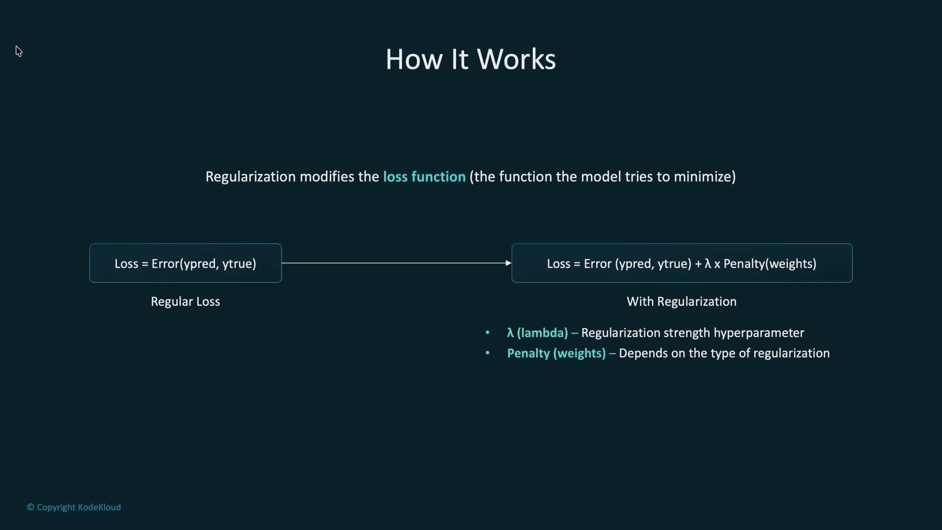
The image explains how regularization modifies the loss function by adding a penalty term to the error, involving a regularization strength hyperparameter (λ) and weight penalty.
Common penalty functions and when to use them:
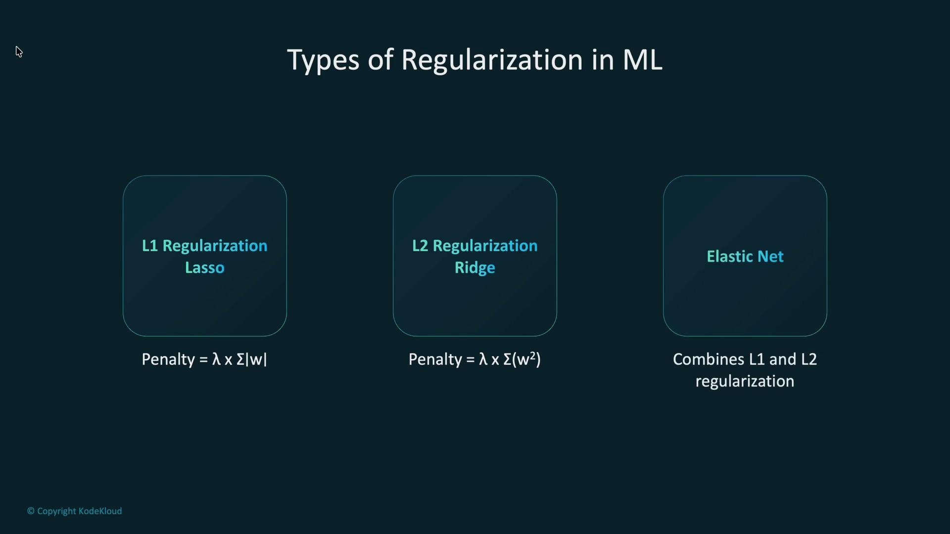
The image depicts three types of regularization in machine learning: L1 (Lasso), L2 (Ridge), and Elastic Net, explaining their penalty calculations.
Scikit-learn examples: Ridge (L2) and Lasso (L1)
Regularization beyond linear models
  • Dropout (deep learning): randomly disables a subset of neurons during each training step, preventing co-adaptation and reducing overfitting.
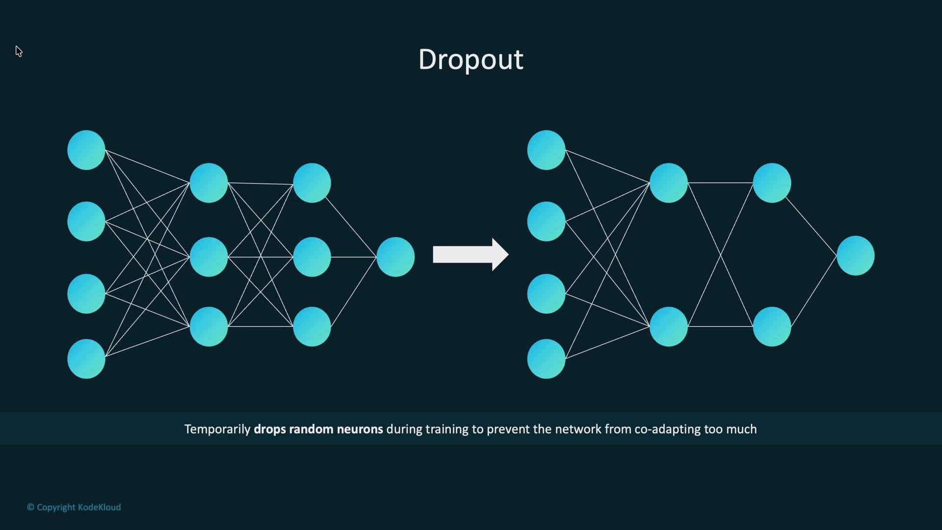
The image illustrates the dropout technique in neural networks, showing network nodes before and after dropout is applied, with some nodes randomly deactivated to prevent co-adaptation.
  • Early stopping: track validation loss or metrics and stop training when improvement stalls to prevent overfitting from excessive epochs.
  • Data augmentation (images): artificially expand training data with random transforms — flips, rotations, crops, brightness/gamma changes — to improve model robustness.
Applying regularization in AWS SageMaker AWS SageMaker built-in algorithms and frameworks expose hyperparameters for common regularization techniques. Use these to control model capacity and generalization when training at scale.
  • Linear Learner supports both L1 and L2:
    • L1: absolute weight penalty, useful for sparsity and feature selection.
    • L2: squared weight penalty, shrinks coefficients to reduce variance.
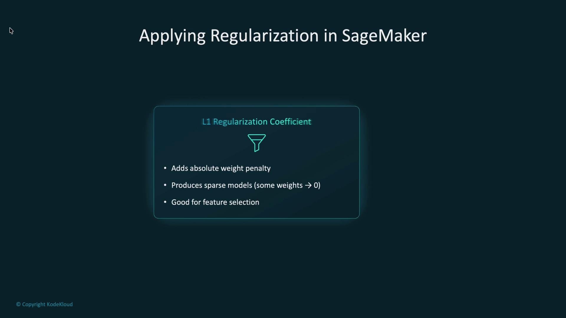
The image is a slide titled "Applying Regularization in SageMaker" describing L1 regularization, which adds an absolute weight penalty, creates sparse models, and is beneficial for feature selection.
Example: Linear Learner via the SageMaker SDK
XGBoost regularization parameters (summary) Example: XGBoost estimator in SageMaker
Other regularization-related training knobs in SageMaker and deep learning:
  • weight_decay: commonly used for L2 regularization.
  • num_layers: increasing layers raises capacity and overfitting risk.
  • mini_batch_size: affects gradient estimates and training stability.
  • epochs: more epochs increase risk of overfitting (use early stopping).
  • learning_rate: impacts optimization dynamics; lower rates can act like a regularizer.
ResNet-based image classification example (SageMaker built-in image classifier)
  • weight_decay implements L2 regularization.
  • learning_rate controls the optimizer behavior (not a regularization parameter, but relevant to convergence).
Tuning regularization strengths
  • Use automated hyperparameter tuning (AWS SageMaker Automatic Model Tuning or other HPO frameworks) to search for optimal values of alpha, lambda, weight_decay, dropout rate, etc.
  • Start with reasonable defaults and sweep logarithmically (e.g., 1e-4 to 1e0) for penalty strengths.
When supplying XGBoost hyperparameters in a Python dict, use string keys for parameters like "lambda" because lambda is a reserved keyword in Python. For example: {"lambda": 1.0}.
Further reading and references Use regularization as part of a broader model-validation strategy: combine cross-validation, monitoring of validation metrics, early stopping, and automated tuning to achieve robust models that generalize well.

Watch Video