ML Algorithms and Business Problem Mapping

Choosing the right machine learning algorithm early shortens time to value: you get usable results faster, ensure the model aligns with business needs, and choose appropriate evaluation metrics. That improves interpretability, operational impact, and the ability to explain and act on model outputs. Machine learning algorithms fall into three main paradigms:

• Supervised learning
• Unsupervised learning
• Reinforcement learning

Each paradigm addresses different problem types and has distinct data and feedback requirements. Overview of the three paradigms:

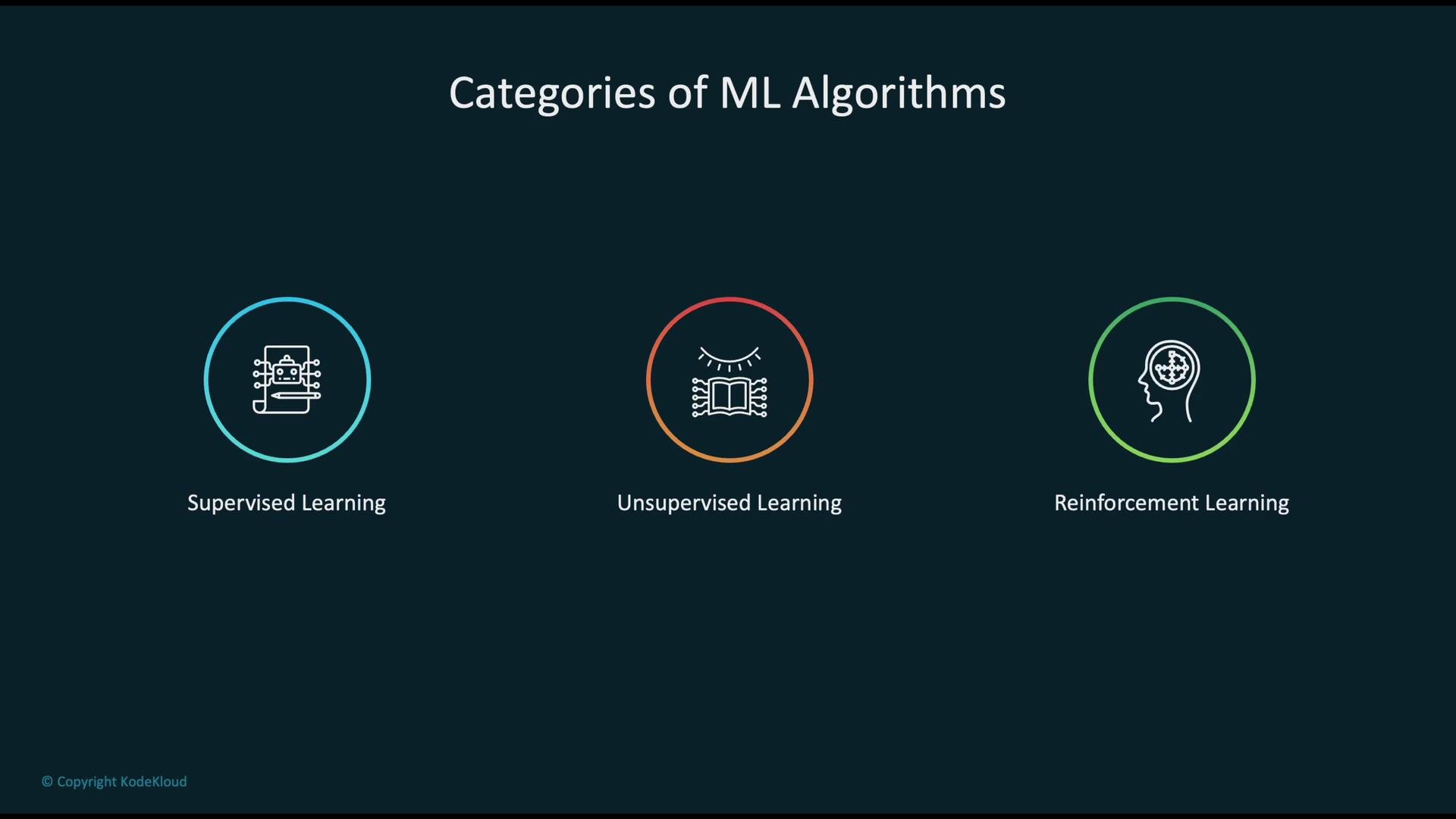
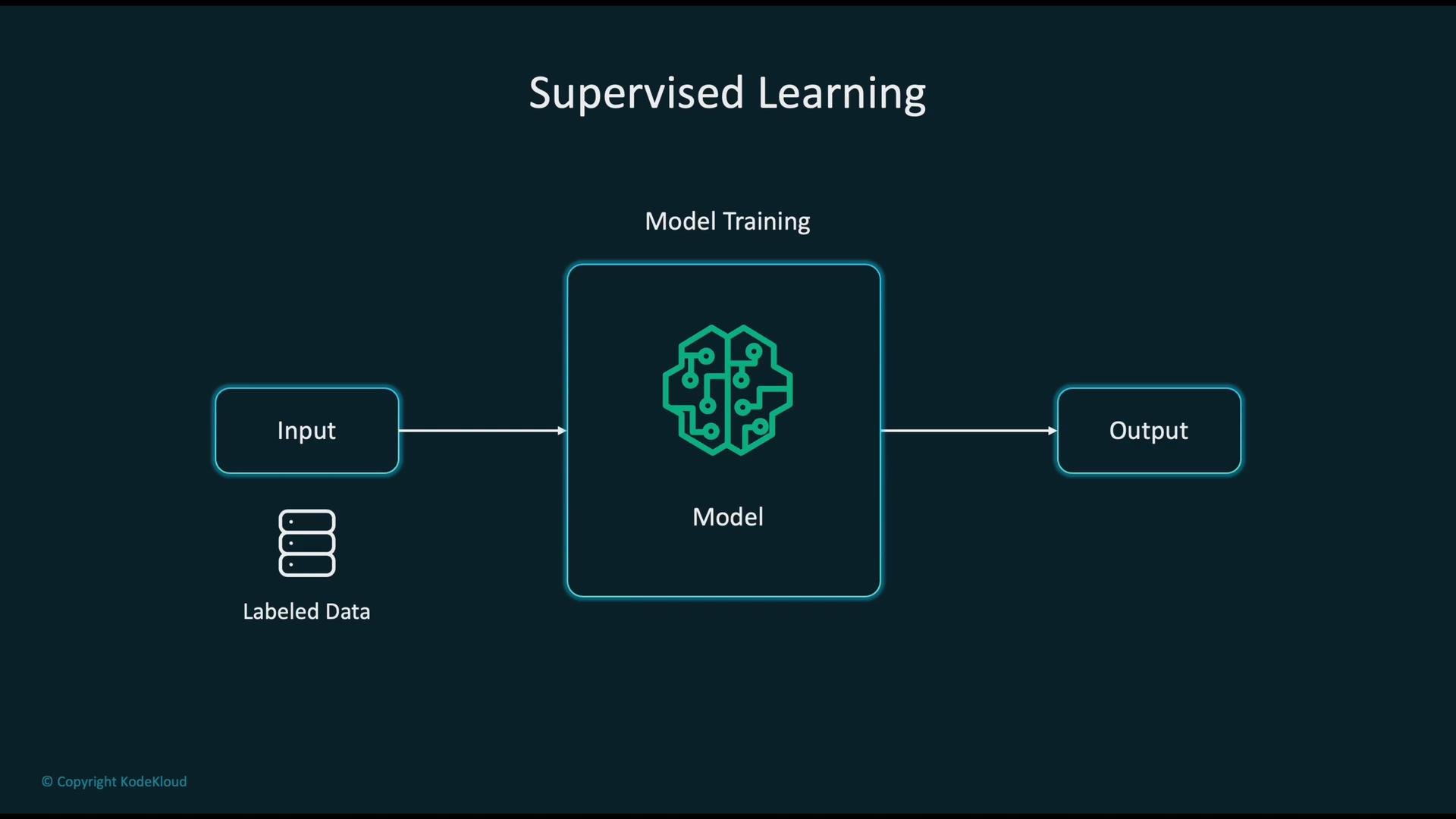
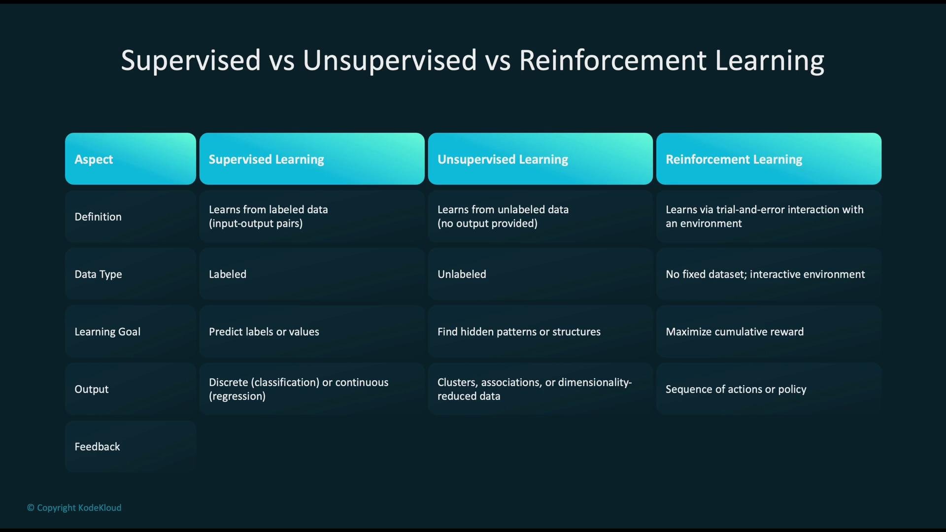
• Supervised learning: Trained on labeled examples (input → correct output). Typical tasks: classification and regression.
• Unsupervised learning: Works with unlabeled data to discover structure or latent representations — e.g., clustering and dimensionality reduction.
• Reinforcement learning: An agent interacts with an environment, learning policies that maximize cumulative reward (applications: robotics, recommendation engines, game AI).

Supervised learning trains models on labeled examples so they learn the mapping from inputs to outputs and generalize to unseen data. Unsupervised learning explores unlabeled datasets to uncover hidden patterns, while reinforcement learning focuses on learning policies (action sequences) that maximize cumulative reward over time. The image below summarizes data type, learning goal, output, and feedback mechanism across paradigms. Quick comparison table (at-a-glance):

---

​

Supervised Learning: Regression vs. Classification

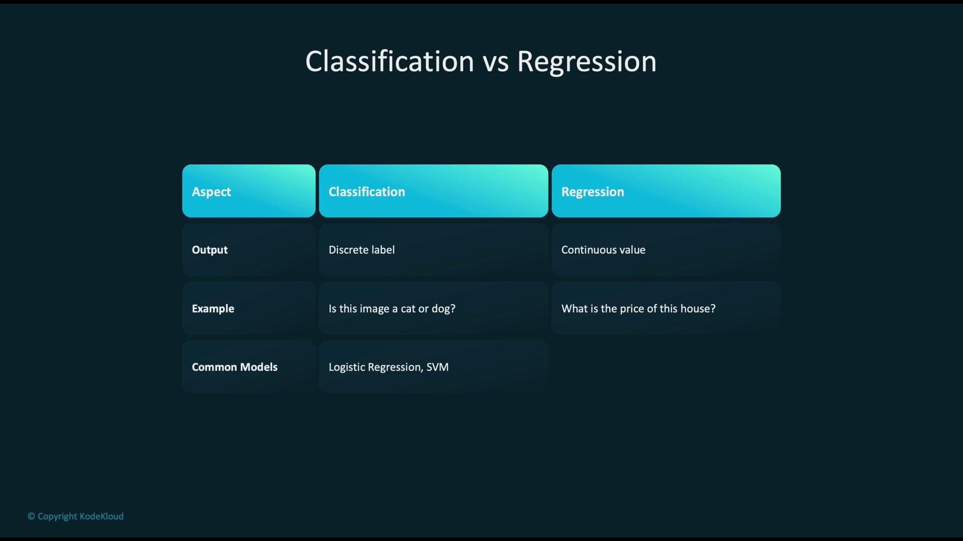
Supervised learning problems split primarily into two categories:

• Regression — predict continuous values (e.g., house prices, temperature).
• Classification — predict discrete labels (e.g., spam vs. not spam, disease vs. healthy).

Regression algorithms (examples and short notes):

• Linear Regression — linear mapping between inputs and output.
• Polynomial Regression — captures nonlinearity via higher-order terms.
• Ridge Regression — linear model with L2 regularization for robustness.
• Lasso Regression — L1 regularization that can produce sparse (feature-selecting) solutions.
• Decision Tree Regression — piecewise constant models via recursive splits.
• Random Forest Regression — ensemble of trees for better accuracy and stability.
• Gradient Boosting (e.g., XGBoost, LightGBM) — strong performance on tabular regression tasks.

Classification predicts categorical outputs. Common problem types:

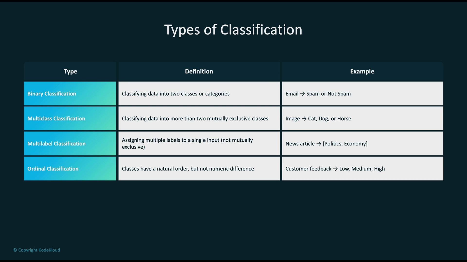
• Binary classification — two classes (e.g., spam vs. not spam).
• Multi-class classification — one label from many mutually exclusive classes.
• Multi-label classification — multiple independent labels per instance.
• Ordinal classification — classes with a meaningful order (e.g., risk levels).
• Nominal classification — unordered categories.

Evaluation metrics differ by task: Common model choices:

---

​

Unsupervised Learning: Clustering and Beyond

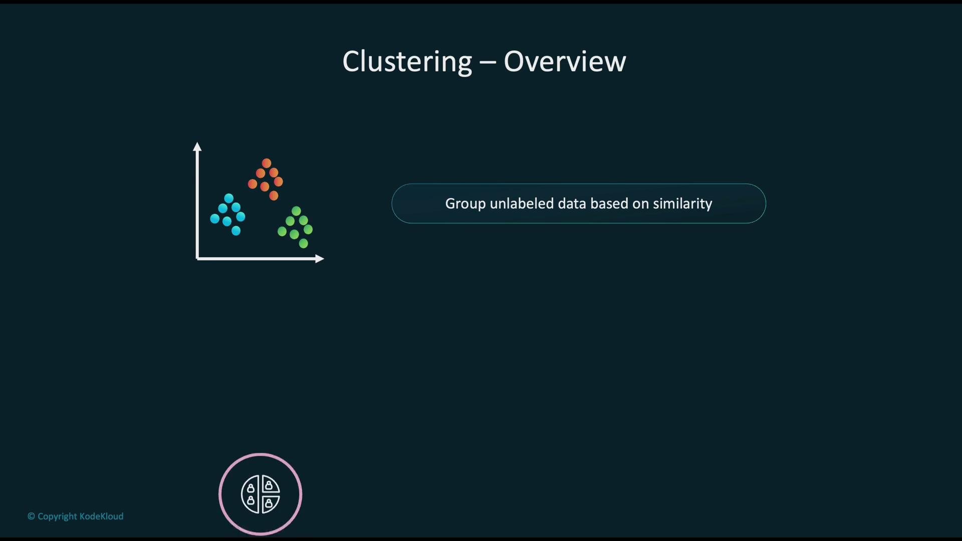
Unsupervised learning extracts structure from unlabeled data. One of the most common tasks is clustering, which groups observations by similarity. Typical use cases include customer segmentation, product grouping, and behavioral profiling. Common clustering algorithms:

• K-means — fast, centroid-based, assumes spherical clusters.
• Hierarchical clustering — builds nested clusters, useful for dendrograms.
• DBSCAN — density-based, identifies arbitrarily-shaped clusters and noise.
• Gaussian Mixture Models — probabilistic clusters with soft assignments.

Another important unsupervised task is dimensionality reduction (PCA, t-SNE, UMAP) for visualization, feature reduction, or denoising.

​

Anomaly Detection

Anomaly detection identifies rare or unexpected events and is widely used in:

• Credit card fraud detection
• Network intrusion detection
• Predictive maintenance (detect equipment failure)
• Medical anomaly detection

Approaches for anomaly detection:

• Statistical thresholding and z-scores
• Isolation Forests — tree-based isolation for outliers
• One-Class SVM — boundary-based approach for normal data
• Autoencoders — reconstruction error flags anomalies

Choose the method based on labeled anomaly examples availability, the expected false-positive rate, and operational constraints (latency, explainability).

---

​

Practical Mapping Checklist

Use this checklist when mapping a business problem to algorithms:

1. Define the objective clearly (classification, regression, clustering, anomaly detection, policy optimization).
2. Identify whether labeled data is available and its quality.
3. Select evaluation metrics aligned with business impact (precision, recall, MAE, revenue-based metrics).
4. Choose model families that suit data size, feature types, and interpretability needs.
5. Prototype with simple baselines (logistic regression, decision trees) before moving to complex models.
6. Monitor models in production for data drift, label shift, and performance degradation.

Relevant resources:

• Kubernetes Documentation (for model deployment patterns)
• Docker Hub (containerizing models)
• Scikit-learn (classical ML algorithms)
• XGBoost / LightGBM (gradient boosting implementations)

By aligning the algorithm choice with the problem type, data characteristics, and evaluation metric early, you accelerate delivery of meaningful, explainable, and actionable ML solutions.