- Autoscaling behavior: streaming vs batch
- Shuffle service trade-offs
- Detecting and mitigating data skew / hot keys
- Streaming Engine: separation of compute and service-managed state
- Cost optimization and periodic design reviews
Autoscaling behavior: streaming vs batch
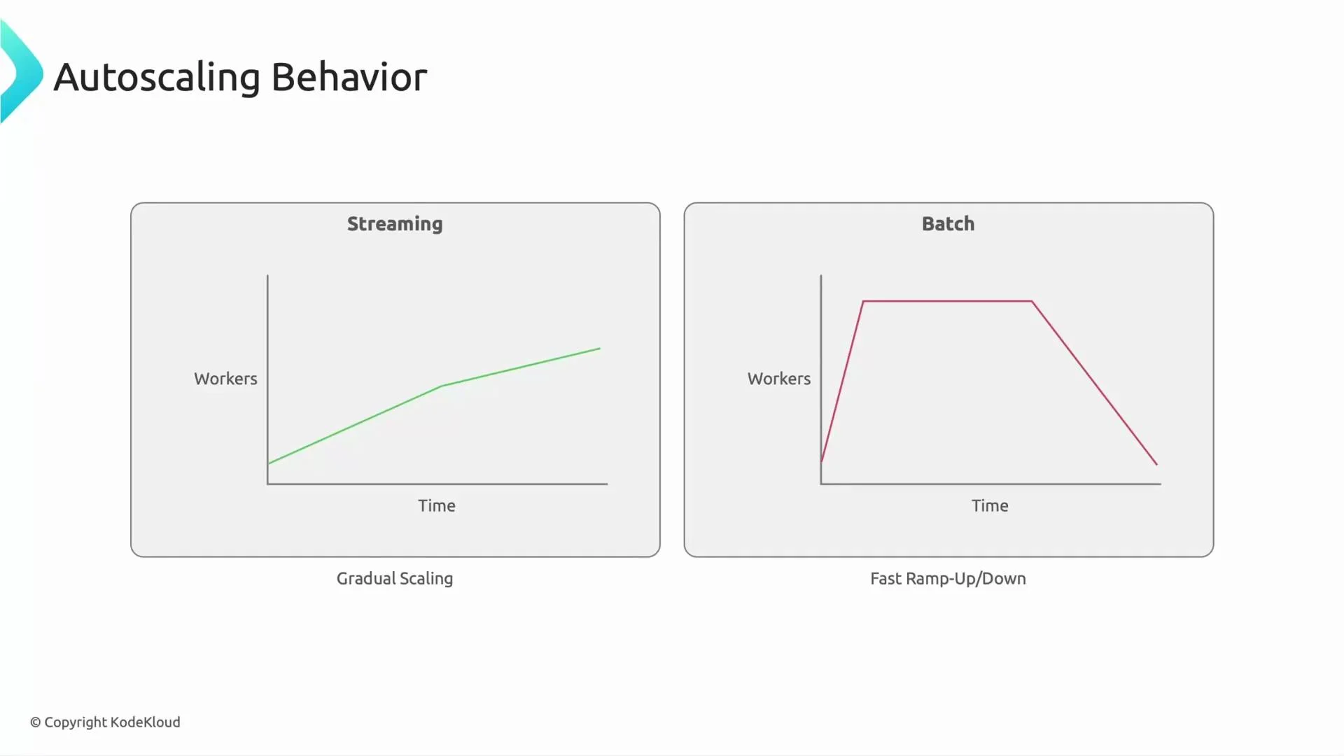
Streaming pipelines run continuously and typically autoscale gradually as load changes. Batch pipelines usually start many workers quickly, process the workload, then scale down when the job completes. These different behaviors imply distinct design and cost trade-offs:- Streaming: steady, incremental autoscaling; optimized for sustained workload and low-latency processing.
- Batch: fast ramp-up and ramp-down; optimized for burst throughput and short-lived runs.
Shuffle service: local disk vs external shuffle
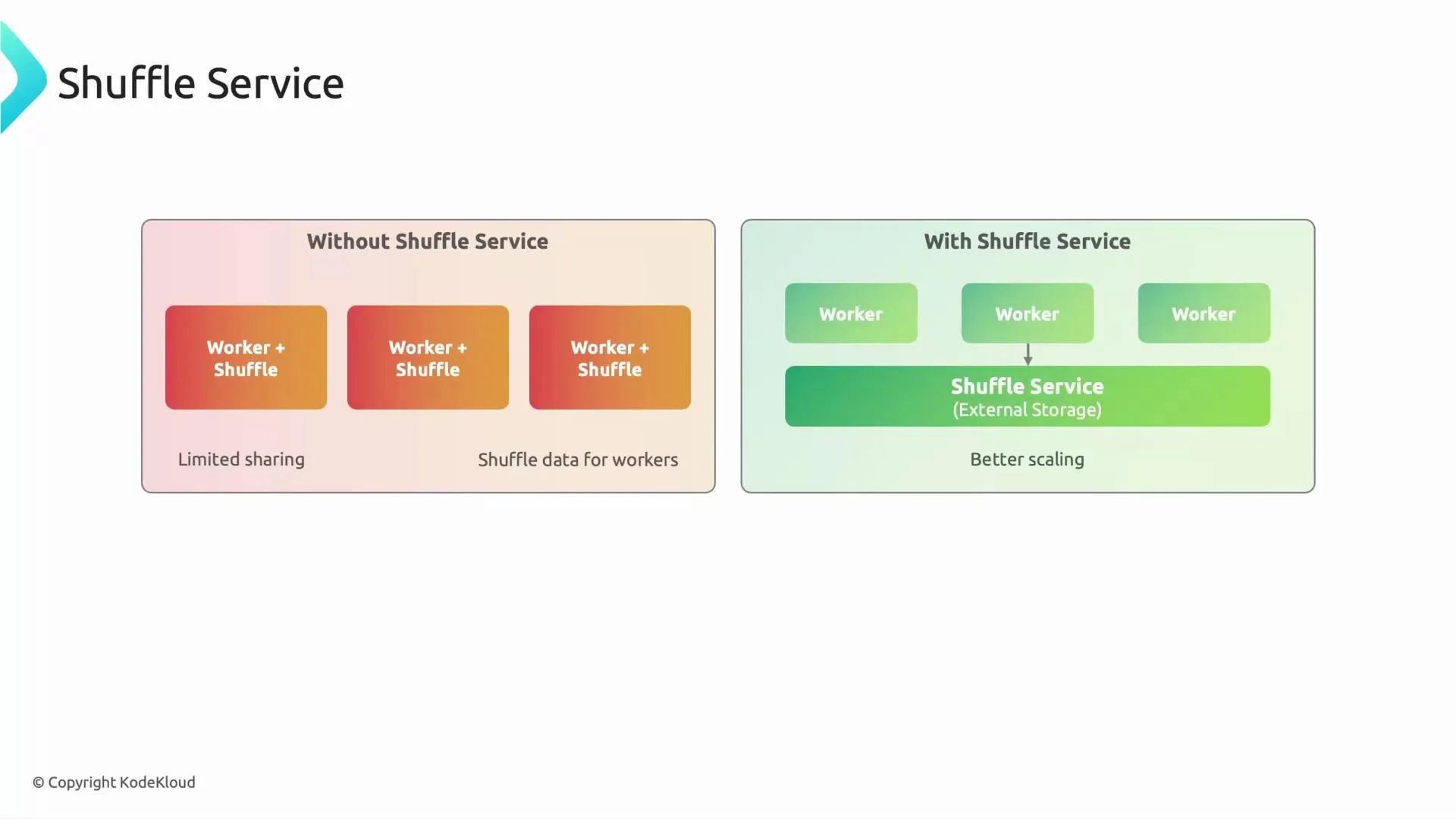
By default, Dataflow can store intermediate shuffle data on worker VMs’ local disks. In this mode, if a worker fails, the stage may need to restart and reprocess lost intermediate data—costly in time and compute. Enabling the Dataflow Shuffle Service stores intermediate data in a separate, resilient service so workers become effectively stateless for intermediate data. A replacement worker can continue from the external shuffle store without reprocessing the entire stage, improving fault tolerance and enabling faster, more reliable scaling. However, the external shuffle service introduces overhead and may not be beneficial for very short-lived batch jobs (e.g., tasks that run for only a minute or two). Evaluate expected job duration, failure tolerance, and cost trade-offs before enabling it.Use the external shuffle service for long-running or failure-sensitive jobs. For tiny, short-lived batch jobs, the external shuffle overhead can increase latency and cost.
Detecting and mitigating data skew / hot keys
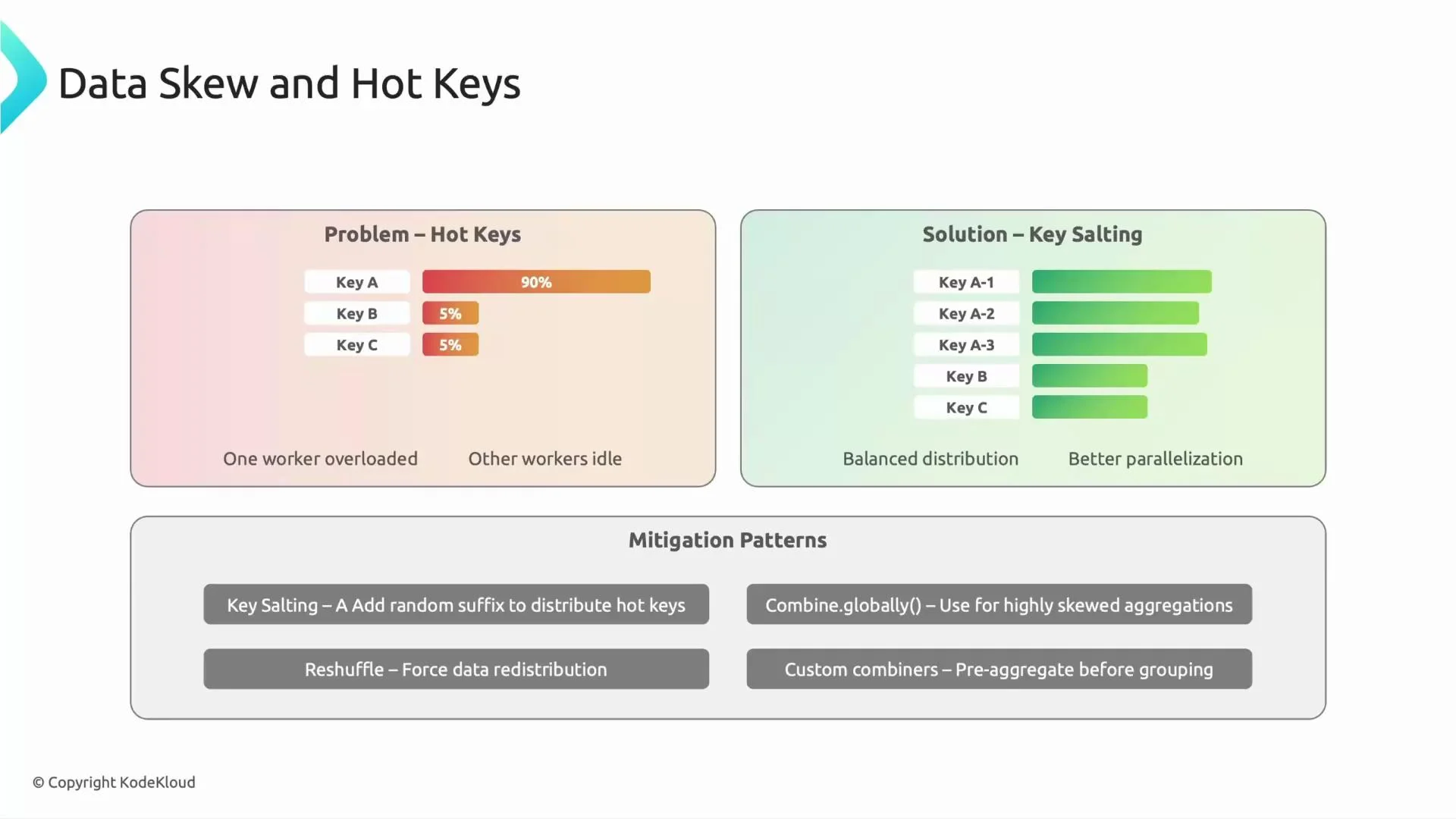
Data skew (hot keys) happens when a small subset of keys receives a disproportionate share of the data. This creates bottlenecks: the worker handling the hot key becomes overloaded while others are idle, reducing parallelism and increasing latency. Common mitigations:- Key salting (sharding / key prefixing): split a hot key into multiple salted keys for partial aggregation, then remove the salt and perform a final aggregation.
- Reshuffle / multi-stage aggregation: perform partial combines (fanout) before a final CombinePerKey.
- Worker-side combining: reduce the amount of shuffle data by aggregating locally where possible.
- Monitor per-key throughput and latency using Dataflow job metrics and logs to identify skew.
- For identified hot keys, implement a two-stage combine pattern:
- Choose the number of shards based on observed load for the hot key (e.g., K-0..K-N).
- Use fanout/combiner patterns to reduce intermediate shuffle volume.
Streaming Engine: separation of compute and service-managed state
Dataflow supports two runtime models:- Legacy worker-centric streaming (worker holds state and coordination),
- Managed Streaming Engine (service-managed state and coordination).
- Faster autoscaling (workers can be added/removed more quickly),
- Lower worker memory footprint,
- Improved worker resource utilization,
- Better support for low-latency, short-interval streaming.
Cost optimization and ongoing design review
Control costs by selecting appropriate machine types, autoscaling settings, and shuffle/engine configurations. Practical ideas:- Right-size worker machine types for CPU and memory needs.
- Use preemptible workers for batch jobs where occasional interruptions are acceptable (significant cost savings).
- Tune autoscaling parameters and set reasonable minimum/maximum worker counts to balance latency and cost.
- Avoid enabling shuffle service for tiny, short-lived jobs where overhead outweighs reliability gains.
- Apply partial aggregation or fanout to reduce shuffle volume and network I/O.
Do a design review at regular intervals (for example, yearly). Re-evaluating pipelines against newer managed services and features often yields both performance and cost benefits.