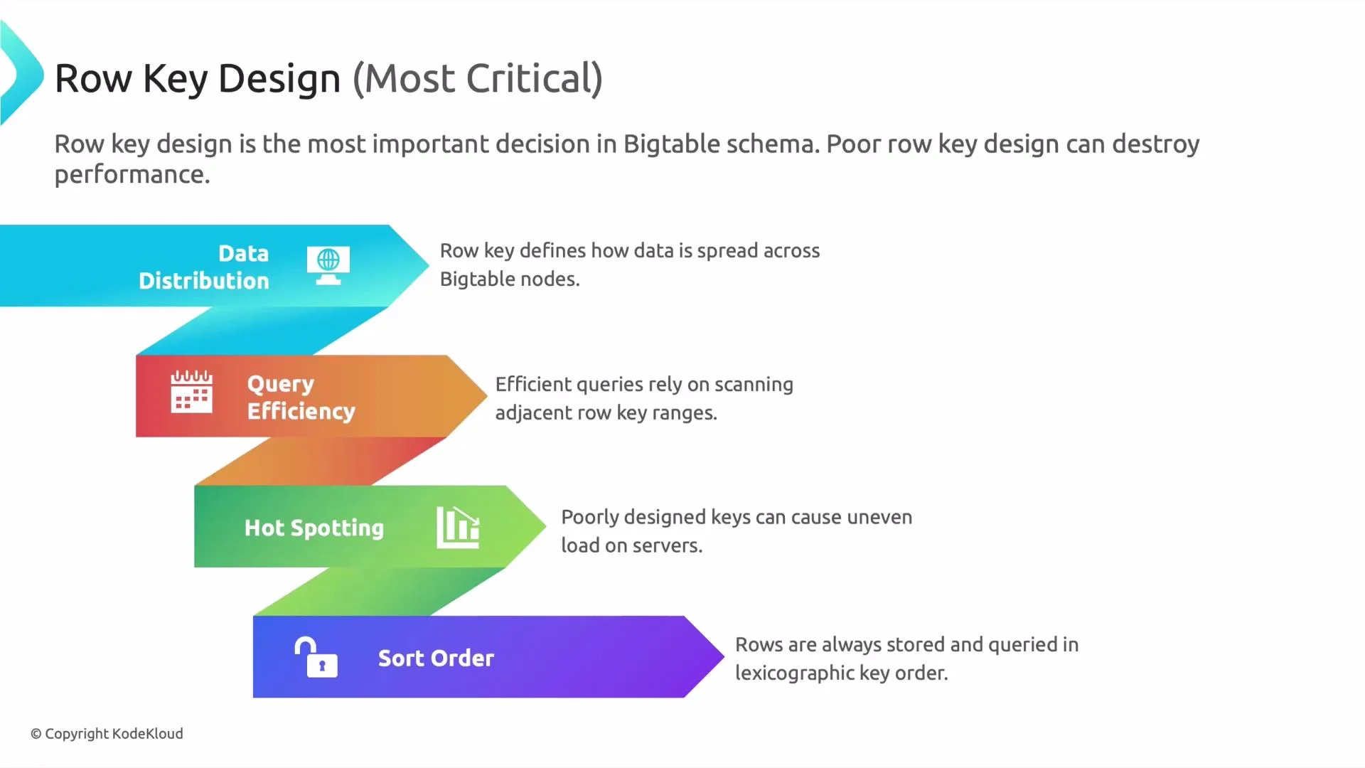
Welcome back. This lesson dives into one of the most critical decisions when using Google Cloud Bigtable: row key design. The row key determines data distribution, query performance, and overall system scalability. A poorly chosen row key can create hotspots, unbalanced tablets, and slow queries—so getting it right is essential. Why row key design matters
  • Data distribution
    The row key controls how Bigtable splits data into tablets and assigns them to nodes. Similar or highly sequential keys can concentrate data on a few tablets, creating uneven resource use.
  • Query efficiency
    Bigtable excels at contiguous range scans. Keys that colocate related rows (for example, via a consistent prefix) make range queries fast and efficient.
  • Hotspotting
    Writes that target the same key range will overload a single tablet. Avoid predictable, strictly increasing keys for high-write workloads.
  • Sort order
    Rows are ordered lexicographically by key. This behavior is ideal for time-series and prefix-based access, but naive timestamp-leading keys will funnel writes to the same tablet.
A typical pitfall: leading timestamps If your row keys start with an increasing timestamp, new rows are always appended at the same end of the lexicographic order. That concentrates writes on one tablet and causes hotspotting. Use hashing, bucketing, or transform timestamps to distribute load.
A presentation slide titled "Row Key Design (Most Critical)" showing a colorful ribbon infographic that lists key Bigtable concerns: Data Distribution, Query Efficiency, Hotspotting, and Sort Order with brief explanations. It emphasizes that poor row key design can destroy performance.
Sensor-data example and six core principles Below we apply row-key and schema principles to a sensor readings scenario and then summarize six core design principles you should follow.
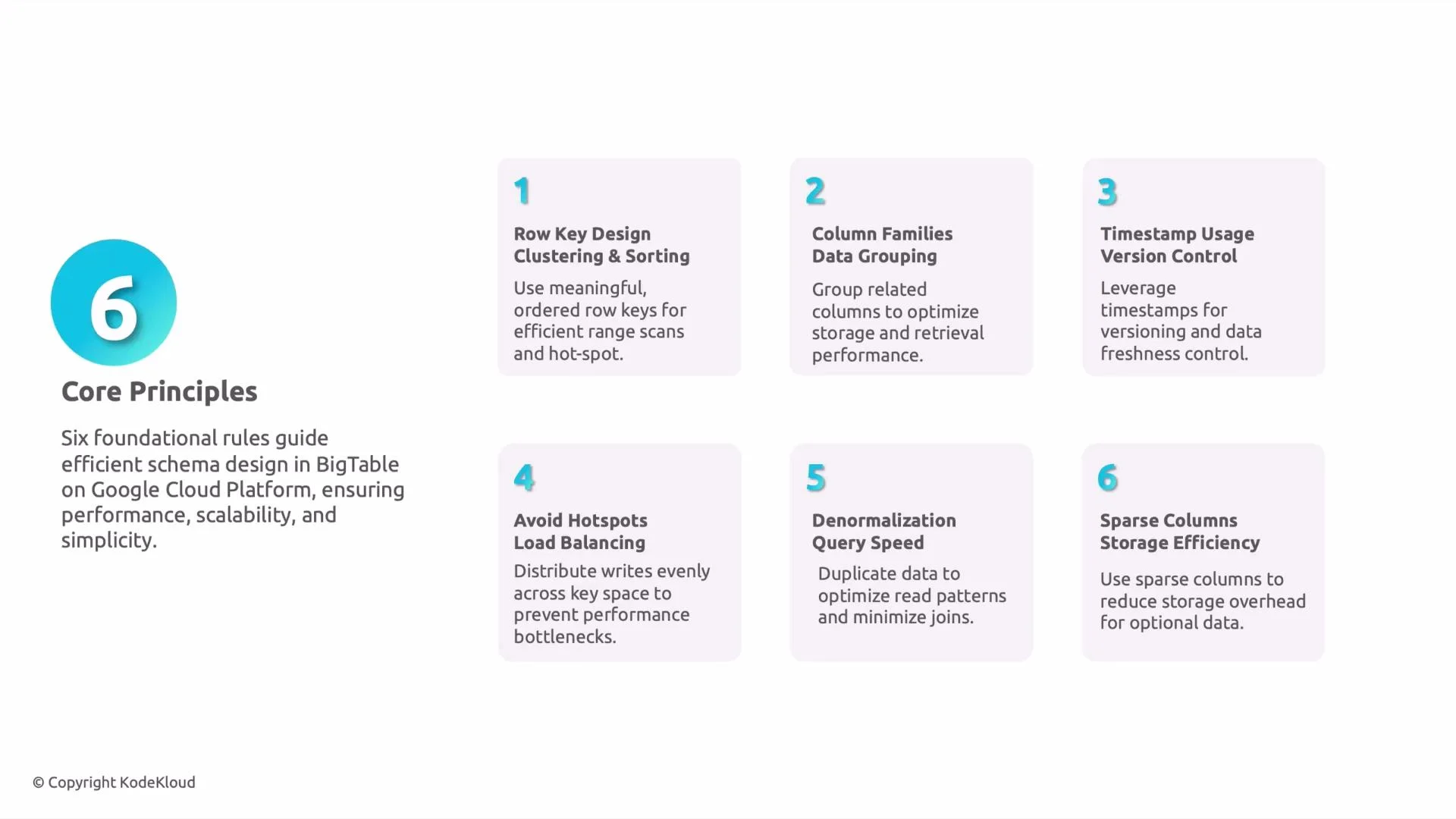
  1. Row key design, clustering, and sort order
  • Use a key layout that groups related rows so range scans are contiguous and efficient.
  • For sensor data, prefix the key with the sensor identifier to cluster that sensor’s readings together.
Good example:
sensor123#2023-05-01T12:00:00Z
sensor123#2023-05-01T12:05:00Z
Bad example (causes hotspotting for sequential timestamps):
2023-05-01T12:00:00Z#sensor123
2023-05-01T12:05:00Z#sensor123
  1. Column families (logical grouping)
  • Group columns that are read together into the same column family so Bigtable reads fewer blocks.
  • Example: store temperature and humidity in one family and system_logs in another to avoid unnecessary IO when you only need sensor readings.
  1. Timestamp usage and versions
  • Bigtable stores multiple versions per cell, ordered by timestamp. Use this for short-term history (e.g., last N readings).
  • Configure column-family GC (max versions, age-based retention) to control storage and retention.
  • Example policy: keep the last 5 versions for a measurement column.
  1. Avoid hotspotting and design for load balance
  • Distribute writes across the key space using short hashed prefixes, explicit shard numbers, or timestamp transforms (e.g., reverse timestamps).
  • Preserve read locality where possible—don’t remove prefixes that you need for range scans.
Examples:
# Hashed prefix (3 shards)
shard-02#sensor123#2023-05-01T12:00:00Z

# Reversed timestamp (MAX_TS - timestamp)
sensor123#(9999999999 - 1682942400)
Exam tip: Questions about avoiding hotspotting usually expect answers mentioning hashing, bucketing, or adding randomness to the row key to distribute writes.
Avoid using strictly increasing values (like leading timestamps) as the first part of the row key for high-write workloads—this is a common cause of hot tablets.
  1. Denormalization for performance
  • Bigtable is optimized for wide rows and single-table access. Duplicate frequently used fields (for example, sensor location or type) inside each row to avoid additional lookups or joins.
  • Trade-off: higher storage costs for much faster read latency.
  1. Storage efficiency and sparse columns
  • Bigtable stores only columns with values; sparse columns do not consume storage for rows that lack them.
  • Put optional or infrequent attributes in separate columns or families to avoid extra IO for common queries.
Principles summary table
PrincipleProblem solvedExample
Row key ordering & clusteringEfficient range scans and localitysensor123#2023-05-01T12:00:00Z
Column familiesReduce IO by grouping commonly-read datameasurements:temperature, logs:system
Timestamps & versionsShort-term history without extra rowsKeep last 5 versions (gc: max_versions=5)
Hotspot avoidancePrevent single-tablet write overloadshard-02#sensor123#... or reversed timestamps
DenormalizationFaster reads, fewer lookupsDuplicate sensor_location in each row
Sparse columnsSave storage and IO for optional fieldsUse separate optional columns per attribute
Monitoring and testing
  • Test with a realistic workload and monitor tablet splits, CPU, and IO in Cloud Monitoring (Stackdriver). Watch for skew in tablet sizes and request rates.
  • If you see hotspots, try introducing hashing or additional shards and re-evaluate read patterns.
Links and references Summary Row key design is the single most important Bigtable schema decision. The right pattern depends on access patterns (point lookups vs. range scans), write volume, retention requirements, and whether you need to prioritize read locality or write distribution. Use these six principles as a checklist: order keys for locality, group columns sensibly, use timestamps and GC settings, avoid hotspotting with bucketing or hashing, denormalize for performance, and exploit sparse columns to save space.
An infographic titled "6 Core Principles" for BigTable schema design with a large blue "6" and brief introductory text on the left. Six numbered panels on the right list principles like row key design, column families, timestamp usage, avoiding hotspots, denormalization, and sparse columns with short explanations.
That concludes this lesson. A concise Bigtable summary that ties these concepts together will follow.

Watch Video